aggregation of spatial objects

spatial aggregation of thematic information in spatial objects

# S3 method for Spatial
aggregate(x, by = list(ID = rep(1, length(x))),
        FUN, ..., dissolve = TRUE, areaWeighted = FALSE)

Arguments

x	object deriving from Spatial, with attributes
by	aggregation predicate; if by is a Spatial object, the geometry by which attributes in x are aggregated; if by is a list, aggregation by attribute(s), see aggregate.data.frame
FUN	aggregation function, e.g. mean; see details
...	arguments passed on to function FUN, unless minDimension is specified, which is passed on to function over
dissolve	logical; should, when aggregating based on attributes, the resulting geometries be dissolved? Note that if x has class SpatialPointsDataFrame, this returns an object of class SpatialMultiPointsDataFrame
areaWeighted	logical; should the aggregation of x be weighted by the areas it intersects with each feature of by? See value.

Value

The aggregation of attribute values of x either over the geometry of by by using over for spatial matching, or by attribute values, using aggregation function FUN.

If areaWeighted is TRUE, FUN is ignored and the area weighted mean is computed for numerical variables, or if all attributes are factors, the area dominant factor level (area mode) is returned. This will compute the gIntersection of x and by; see examples below.

If by is missing, aggregates over all features.

Details

FUN should be a function that takes as first argument a vector, and that returns a single number. The canonical examples are mean and sum. Counting features is obtained when summing an attribute variable that has the value 1 everywhere.

Note

uses over to find spatial match if by is a Spatial object

Examples

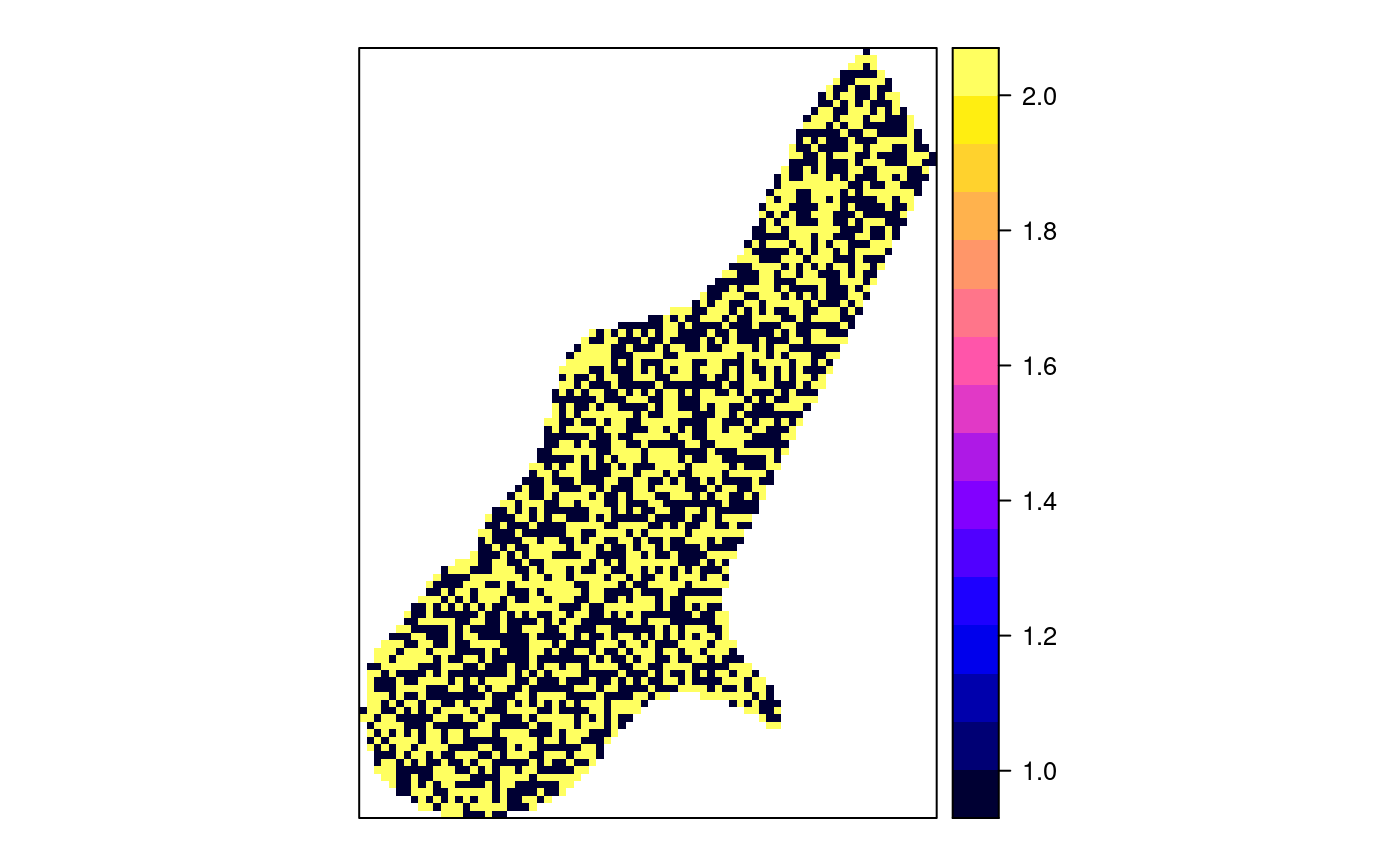
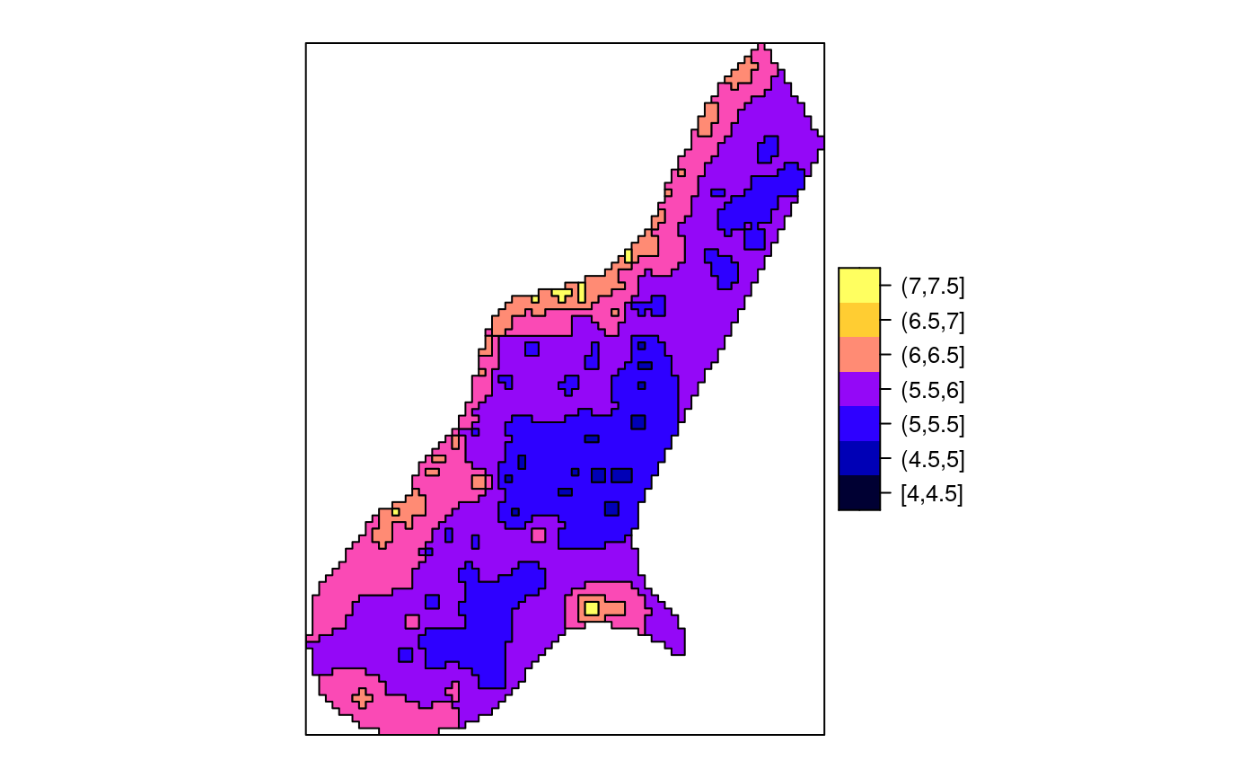
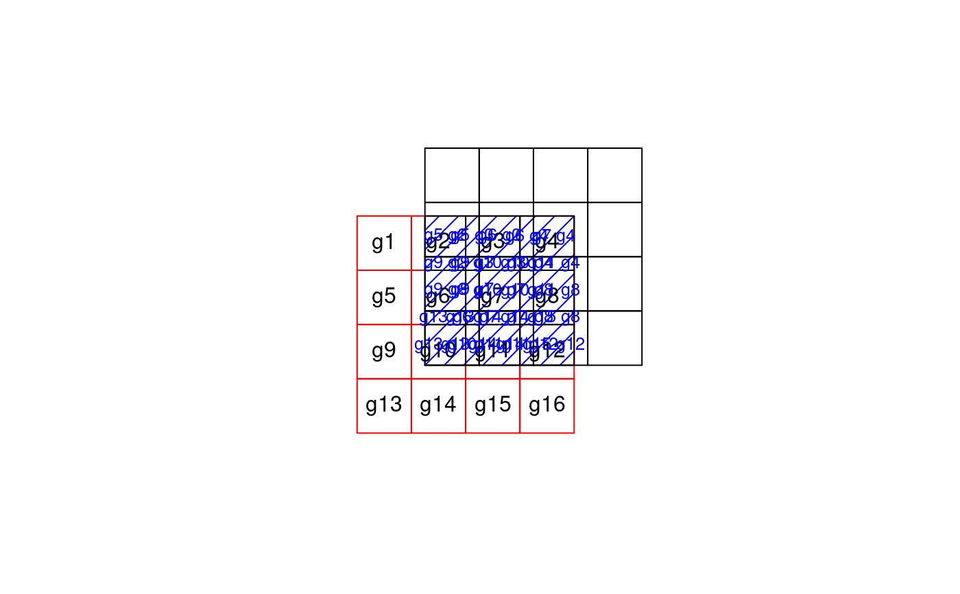
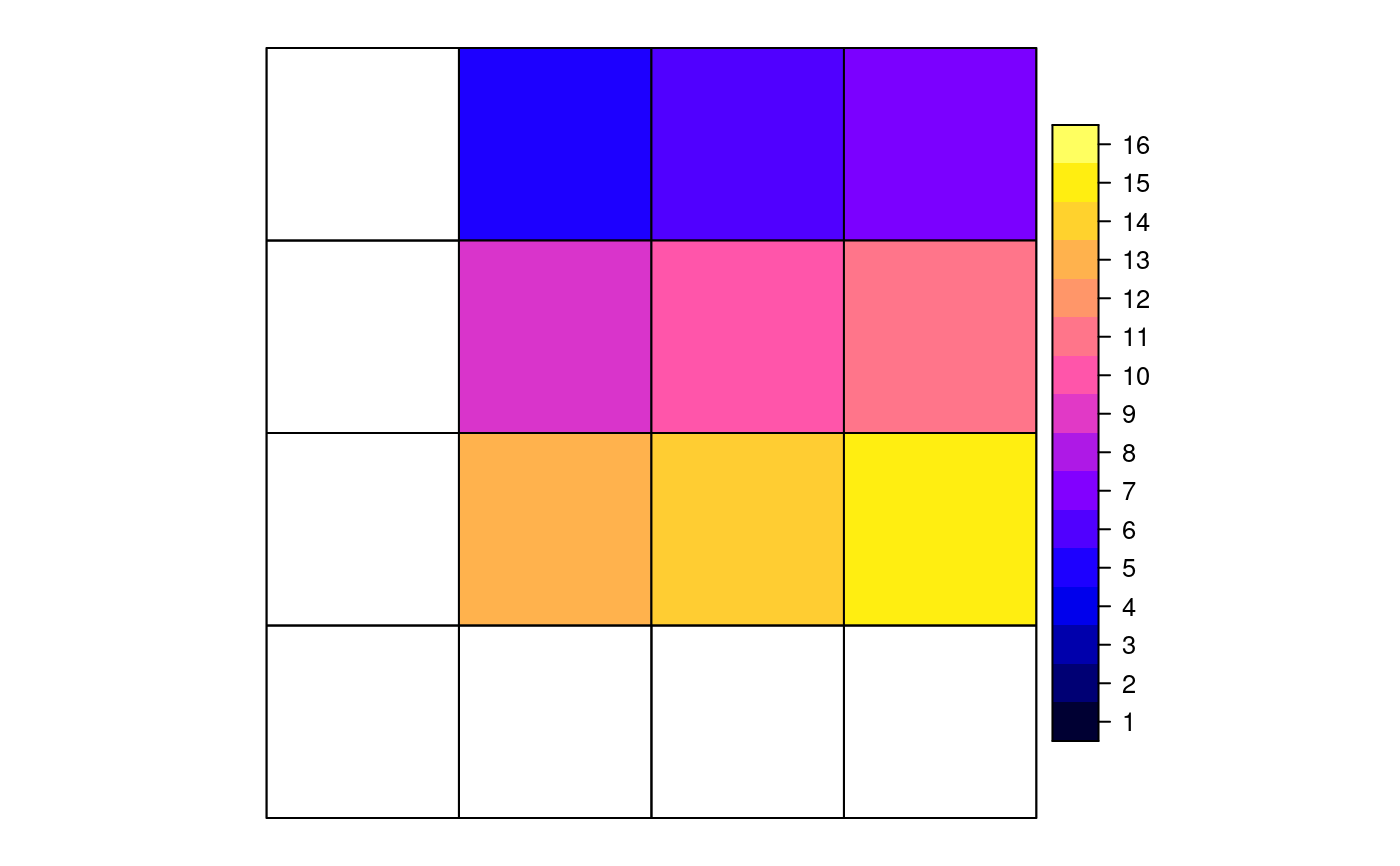
data("meuse")
coordinates(meuse) <- ~x+y
data("meuse.grid")
coordinates(meuse.grid) <- ~x+y
gridded(meuse.grid) <- TRUE
i = cut(meuse.grid$dist, c(0,.25,.5,.75,1), include.lowest = TRUE)
j = sample(1:2, 3103,replace=TRUE)
if (FALSE) {
if (require(rgeos)) {
        # aggregation by spatial object:
        ab = gUnaryUnion(as(meuse.grid, "SpatialPolygons"), meuse.grid$part.a)
        x = aggregate(meuse["zinc"], ab, mean)
        spplot(x)
        # aggregation of multiple variables
        x = aggregate(meuse[c("zinc", "copper")], ab, mean)
        spplot(x)
        # aggregation by attribute, then dissolve to polygon:
        x = aggregate(meuse.grid["dist"], list(i=i), mean)
        spplot(x["i"])
        x = aggregate(meuse.grid["dist"], list(i=i,j=j), mean)
        spplot(x["dist"], col.regions=bpy.colors())
        spplot(x["i"], col.regions=bpy.colors(4))
        spplot(x["j"], col.regions=bpy.colors())
}
}

x = aggregate(meuse.grid["dist"], list(i=i,j=j), mean, dissolve = FALSE)
spplot(x["j"], col.regions=bpy.colors())

if (require(gstat) && require(rgeos)) {
        x = idw(log(zinc)~1, meuse, meuse.grid, debug.level=0)[1]
        spplot(x[1],col.regions=bpy.colors())
        i = cut(x$var1.pred, seq(4, 7.5, by=.5),
                include.lowest = TRUE)
        xa = aggregate(x["var1.pred"], list(i=i), mean)
        spplot(xa[1],col.regions=bpy.colors(8))
}
#> Loading required package: gstat
#> Loading required package: rgeos
#> rgeos version: 0.5-3, (SVN revision 634)
#>  GEOS runtime version: 3.8.1-CAPI-1.13.3 
#>  Linking to sp version: 1.4-1 
#>  Polygon checking: TRUE 

if (require(rgeos)) {
# Area-weighted example, using two partly overlapping grids:

  gt1 = SpatialGrid(GridTopology(c(0,0), c(1,1), c(4,4)))
  gt2 = SpatialGrid(GridTopology(c(-1.25,-1.25), c(1,1), c(4,4)))

  # convert both to polygons; give p1 attributes to aggregate
  p1 = SpatialPolygonsDataFrame(as(gt1, "SpatialPolygons"),
                  data.frame(v = 1:16, w=5:20, x=factor(1:16)), match.ID = FALSE)
  p2 = as(gt2, "SpatialPolygons")

  # plot the scene:
  plot(p1, xlim = c(-2,4), ylim = c(-2,4))
  plot(p2, add = TRUE, border = 'red')
  i = gIntersection(p1, p2, byid = TRUE)
  plot(i, add=TRUE, density = 5, col = 'blue')
  # plot IDs p2:
  ids.p2 = sapply(p2@polygons, function(x) slot(x, name = "ID"))
  text(coordinates(p2), ids.p2)
  # plot IDs i:
  ids.i = sapply(i@polygons, function(x) slot(x, name = "ID"))
  text(coordinates(i), ids.i, cex = .8, col = 'blue')

  # compute & plot area-weighted average; will warn for the factor
  ret = aggregate(p1, p2, areaWeighted = TRUE)
  spplot(ret)

  # all-factor attributes: compute area-dominant factor level:
  ret = aggregate(p1["x"], p2, areaWeighted = TRUE)
  spplot(ret)
}
#> Warning: for factor aggregation, provide factor only data
#> Warning: ‘*’ not meaningful for factors