Class

Class for spatial attributes that have spatial locations on a (full) regular grid.

Objects from the Class

Objects can be created by calls of the form as(x, "SpatialGridDataFrame"), where x is of class SpatialPixelsDataFrame-class, or by importing through rgdal. Ordered full grids are stored instead or unordered non-NA cells;

Slots

grid:

see GridTopology-class; grid parameters

bbox:

Object of class "matrix"; bounding box

proj4string:

Object of class "CRS"; projection

data:

Object of class data.frame, containing attribute data

Extends

Class "SpatialGrid", directly. Class "Spatial", by class "SpatialGrid".

Methods

coordinates

signature(x = "SpatialGridDataFrame"): retrieves (and calculates!) coordinates

[

signature(x = "SpatialGridDataFrame"): selects rows, columns, and attributes; returns an object of class SpatialGridDataFrame

as.matrix

signature(x = "SpatialGridDataFrame"): coerce to matrix; increasing col index corresponds to decreasing y coordinate, row index increases with coordinate index

as.array

signature(x = "SpatialGridDataFrame"): coerce to array; increasing array index for the second dimension corresponds to decreasing coordinates, all other coordinate dimensions increase with array index

cbind

signature(...): if arguments have identical topology, combine their attribute values

Plot method arguments

The plot methods for “SpatialPixelsDataFrame” or “SpatialGridDataFrame” objects take the following arguments:

object of class SpatialPixelsDataFrame or SpatialGridDataFrame

...

arguments passed on to image.SpatialGridDataFrame

attr

integer or character, indicating the attribute variable to be plotted; default 1

col

color ramp to be used; default bpy.colors(100) for continuous, or RColorBrewer::brewer.pal(nlevels(x[[1]]), "Set2") for factor variables

breaks

for continuous attributes: values at which color breaks should take place

zlim

for continuous attributes: numeric of length 2, specifying the range of attribute values to be plotted; default to data range range(as.numeric(x[[attr]])[is.finite(x[[attr]])])

axes

logical: draw x and y axes? default FALSE

xaxs

character, default "i", see par

yaxs

character, default equal to xaxs, see par

numeric or NULL, values at which axis tics and labels should be drawn; default NULL (use pretty)

border

color, to be used for drawing grid lines; default NA (don't draw grid lines)

axis.pos

integer, 1-4; default 4, see axis

add.axis

logical: draw axis along scale? default TRUE

what

what to draw: "image", "scale", or "both"; default "both"

scale.size

size for the scale bar; use lcm to specify in absolute size, or a numeric value such as 1/6 to specify relative size; default lcm(2.8)

scale.shrink

non-negative numeric indicating the amount to shrink the scale length, default 0

scale.frac

for categorical attributes: numeric between 0 and 1, indicating the scale width, default 0.3

scale.n

for categorical attributes: integer, indicating how many scale categories should fill a complete width; default 15

Examples

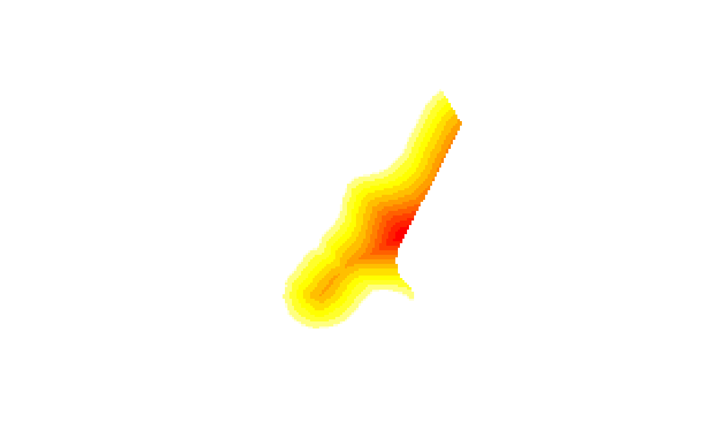
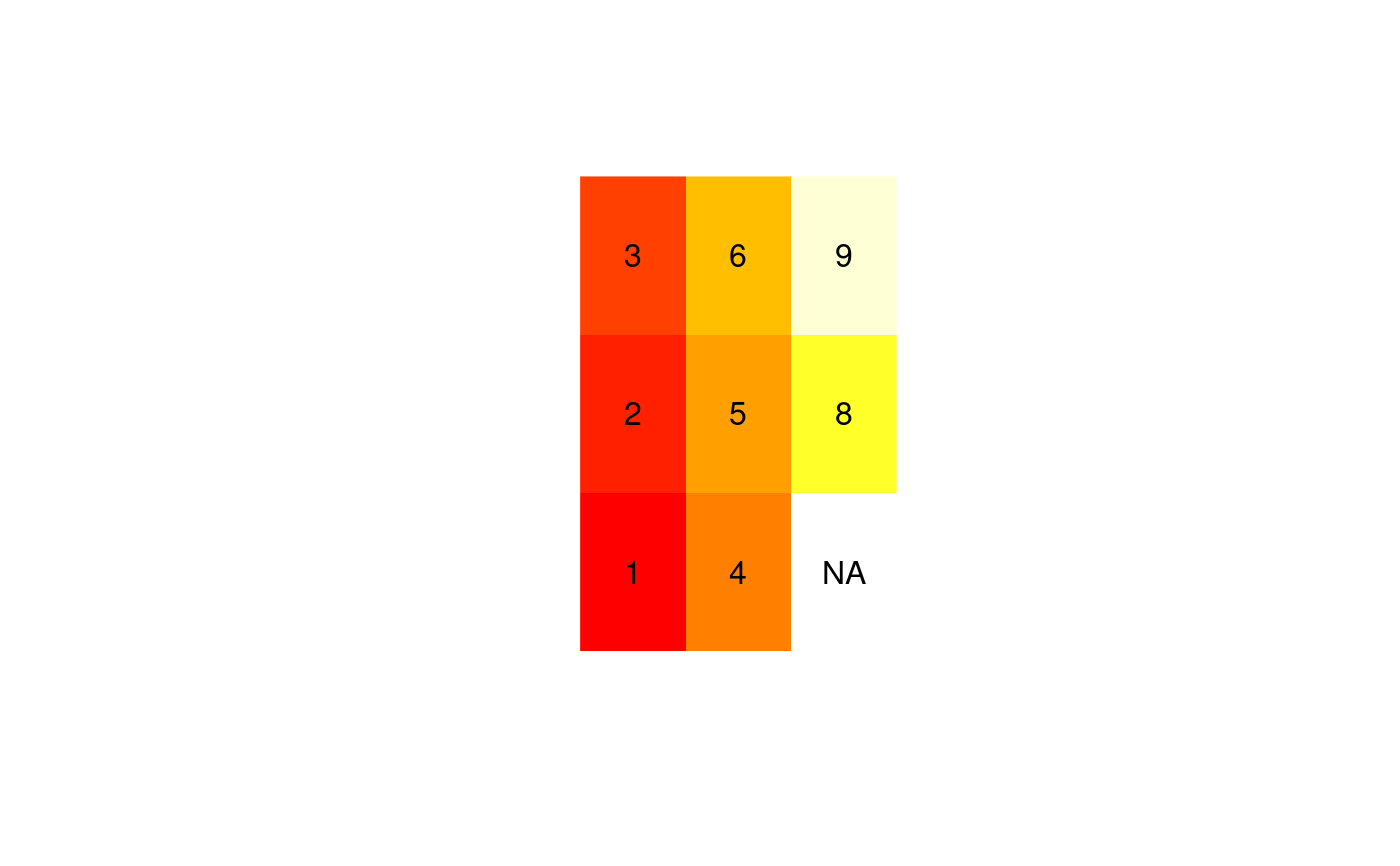
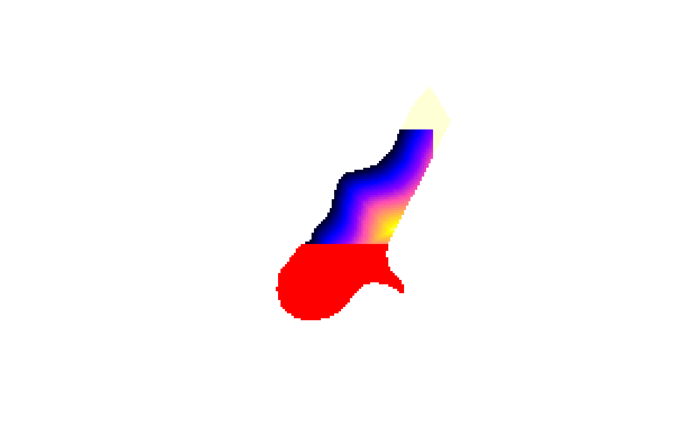
data(meuse.grid) # only the non-missing valued cells
coordinates(meuse.grid) = c("x", "y") # promote to SpatialPointsDataFrame
gridded(meuse.grid) <- TRUE # promote to SpatialPixelsDataFrame
x = as(meuse.grid, "SpatialGridDataFrame") # creates the full grid
x[["idist"]] = 1 - x[["dist"]] # assigns new attribute
image(x["idist"]) # note the single [ for attribute selection

# toy example:
df = data.frame(z = c(1:6,NA,8,9),
    xc = c(1,1,1,2,2,2,3,3,3),
    yc = c(rep(c(0, 1.5, 3),3)))
coordinates(df) = ~xc+yc
gridded(df) = TRUE
df = as(df, "SpatialGridDataFrame") # to full grid
image(df["z"])
# draw labels to verify:
cc = coordinates(df)
z=df[["z"]]
zc=as.character(z)
zc[is.na(zc)]="NA"
text(cc[,1],cc[,2],zc)

# the following is weird, but illustrates the concept of row/col selection:
fullgrid(meuse.grid) = TRUE
image(meuse.grid)
image(meuse.grid[20:70, 10:70, "dist"], add = TRUE, col = bpy.colors())

# as.matrix, as.array
sgdim = c(3,4)
SG = SpatialGrid(GridTopology(rep(0,2), rep(10,2), sgdim))
SGDF = SpatialGridDataFrame(SG, data.frame(val = 1:12))
as.array(SGDF)
#>      [,1] [,2] [,3] [,4]
#> [1,]    1    4    7   10
#> [2,]    2    5    8   11
#> [3,]    3    6    9   12
as.matrix(SGDF)
#>      [,1] [,2] [,3] [,4]
#> [1,]    1    4    7   10
#> [2,]    2    5    8   11
#> [3,]    3    6    9   12
as(SGDF, "array")
#>      [,1] [,2] [,3] [,4]
#> [1,]    1    4    7   10
#> [2,]    2    5    8   11
#> [3,]    3    6    9   12