library(rgugik)
library(sf)Linking to GEOS 3.12.1, GDAL 3.9.0, PROJ 9.4.0; sf_use_s2() is TRUEsubstring(commune_names$TERYT, 1, 2) -> vpom
commune_names |> subset(subset = vpom == "22") -> pom0As was mentioned above in section Section 2.1, spatial vector geometries are most often furnished with identification keys, permitting other data using the same key or index identifiers to be added correctly. In Poland, they have been known as "TERYT", and are fairly stable over time, though border changes can occur, with new key values appearing and old values ceasing to be used, leading to breaks of series. The rgugik package contains a data object listing these keys together with unit names, but matching on names can be troublesome. First we will subset this object to the Pomeranian voivodeship:
library(rgugik)
library(sf)Linking to GEOS 3.12.1, GDAL 3.9.0, PROJ 9.4.0; sf_use_s2() is TRUEsubstring(commune_names$TERYT, 1, 2) -> vpom
commune_names |> subset(subset = vpom == "22") -> pom0then retrieve the boundaries of municipalities in Pomerania using "TERYT" rather than using the names of municipalities, which are duplicated in other voivodeships:
borders_get(TERYT = pom0$TERYT) -> pomMerging the pom object containing the "TERYT" keys and municipality names, with pom_sf, including the "TERYT" keys and municipality boundaries is easy, as the keys are both character objects - this matters because some keys may start with 0, zero, and be wrongly read as integers, dropping leading zeros. The key for this voivodeship is "22", so this problem is not encountered here, but often occurs. Should an identifying key with leading zeros be read as integer, it can be restored using base::formatC after checking the required string width:
ID <- as.integer("0012345")
str(ID) int 12345formatC(ID, format="d", width=7, flag="0")[1] "0012345"Note that the "TERYT" key values returned in the pom_sf object include an underscore between the six digit territorial code and the trailing digit expressing the type of municipality.
dim(pom)[1] 123 2pom |> sapply(class) |> str()List of 2
$ TERYT: chr "character"
$ geom : chr [1:2] "sfc_MULTIPOLYGON" "sfc"str(pom$TERYT) chr [1:123] "226401_1" "221101_1" "221106_2" "220605_2" "221207_2" ...str(pom0)Classes 'tbl_df', 'tbl' and 'data.frame': 123 obs. of 2 variables:
$ NAME : chr "Sopot" "Hel" "Krokowa" "Liniewo" ...
$ TERYT: chr "2264011" "2211011" "2211062" "2206052" ...The underscore needs to be removed before finally checking that they match:
pom$TERYT <- sub("_", "", pom$TERYT)
any(is.na(match(pom$TERYT, pom0$TERYT)))[1] FALSEFinally, the merging operation may be carried out:
pom |> merge(pom0, by = "TERYT") -> pom1
pom1Simple feature collection with 123 features and 2 fields
Geometry type: MULTIPOLYGON
Dimension: XY
Bounding box: xmin: 350809.9 ymin: 626314.8 xmax: 542048.1 ymax: 775019.1
Projected CRS: ETRF2000-PL / CS92
First 10 features:
TERYT NAME geometry
1 2201012 Borzytuchom MULTIPOLYGON (((392568.1 69...
2 2201023 Bytów MULTIPOLYGON (((399745.2 68...
3 2201032 Czarna Dąbrówka MULTIPOLYGON (((415365.5 72...
4 2201042 Kołczygłowy MULTIPOLYGON (((382369 6921...
5 2201052 Lipnica MULTIPOLYGON (((392500.3 67...
6 2201063 Miastko MULTIPOLYGON (((366331.6 67...
7 2201072 Parchowo MULTIPOLYGON (((414238.3 69...
8 2201082 Studzienice MULTIPOLYGON (((405862.1 68...
9 2201092 Trzebielino MULTIPOLYGON (((376562.5 69...
10 2201102 Tuchomie MULTIPOLYGON (((384623.5 68...Having methodically made a first merge, we can move forward with three files at the municipality level from Statistics Poland’s local data bank. These were exported as comma (or semicolon) separated value (CSV) files on February 15, 2024 - dates matter, as online data banks update their contents as inaccuracies are detected. Currently, no package provides direct access to this data bank, and for moderate data volumes, registration is required. The first file is semicolon separated, and contains population data by age group and sex (category K3, group G7, subgroup P2577) for the end of the second half-year 2022:
pop22 <- read.csv("Datasets/sd/LUDN_2577_2022.csv", sep=";")As with most such data, the column names need adjustment. On reading, reserved characters in R are replaced by dots, and for further work, shorter column names are helpful. Current R versions support multibyte characters across all platforms, but some files with single-byte characters can be encountered, in which case judicious use of base::iconv may be needed.
sapply(pop22, class) Kod
"integer"
Nazwa
"character"
w.wieku.przedprodukcyjnym...14.lat.i.mniej.mężczyźni.2022..osoba.
"integer"
w.wieku.przedprodukcyjnym...14.lat.i.mniej.kobiety.2022..osoba.
"integer"
w.wieku.produkcyjnym..15.59.lat.kobiety..15.64.lata.mężczyźni.mężczyźni.2022..osoba.
"integer"
w.wieku.produkcyjnym..15.59.lat.kobiety..15.64.lata.mężczyźni.kobiety.2022..osoba.
"integer"
w.wieku.poprodukcyjnym.mężczyźni.2022..osoba.
"integer"
w.wieku.poprodukcyjnym.kobiety.2022..osoba.
"integer"
X
"logical" pop22$Kod <- as.character(pop22$Kod)
names(pop22)[3:8] <- c("m_u15", "f_u15",
"m_15_64", "f_15_59", "m_o65", "k_o60")
pop22$type <- factor(substring(pop22$Kod, 7, 7),
levels = c("1", "2", "3"),
labels = c("urban", "rural", "urban_rural"))
names(pop22) [1] "Kod" "Nazwa" "m_u15" "f_u15" "m_15_64" "f_15_59" "m_o65"
[8] "k_o60" "X" "type" The key column was read as integer, so needs correcting; otherwise the remaining columns seem to be formatted acceptably. A new column is created as a factor showing the type of municipality, as a factor In addition, we The "X" column contains no data, and is dropped from the merging operation. We could overwrite the cumulating object on merge; here we choose to create a new object at each merge. The key is called "TERYT" in pom_sf and "Kod" in pop92, specified with by.x and by.y arguments:
pom1 |> merge(pop22[, -9], by.x = "TERYT",
by.y = "Kod") -> pom2
pom2Simple feature collection with 123 features and 10 fields
Geometry type: MULTIPOLYGON
Dimension: XY
Bounding box: xmin: 350809.9 ymin: 626314.8 xmax: 542048.1 ymax: 775019.1
Projected CRS: ETRF2000-PL / CS92
First 10 features:
TERYT NAME Nazwa m_u15 f_u15 m_15_64 f_15_59
1 2201012 Borzytuchom Borzytuchom (2) 406 387 1181 1039
2 2201023 Bytów Bytów (3) 2306 2162 8236 7373
3 2201032 Czarna Dąbrówka Czarna Dąbrówka (2) 610 596 1859 1556
4 2201042 Kołczygłowy Kołczygłowy (2) 387 308 1425 1203
5 2201052 Lipnica Lipnica (2) 531 449 1702 1463
6 2201063 Miastko Miastko (3) 1424 1331 6058 5021
7 2201072 Parchowo Parchowo (2) 416 382 1237 1106
8 2201082 Studzienice Studzienice (2) 346 352 1206 1066
9 2201092 Trzebielino Trzebielino (2) 350 299 1213 998
10 2201102 Tuchomie Tuchomie (2) 400 366 1462 1265
m_o65 k_o60 type geometry
1 172 301 rural MULTIPOLYGON (((392568.1 69...
2 1794 3250 urban_rural MULTIPOLYGON (((399745.2 68...
3 406 657 rural MULTIPOLYGON (((415365.5 72...
4 293 464 rural MULTIPOLYGON (((382369 6921...
5 389 611 rural MULTIPOLYGON (((392500.3 67...
6 1430 2773 urban_rural MULTIPOLYGON (((366331.6 67...
7 243 414 rural MULTIPOLYGON (((414238.3 69...
8 249 406 rural MULTIPOLYGON (((405862.1 68...
9 250 446 rural MULTIPOLYGON (((376562.5 69...
10 270 420 rural MULTIPOLYGON (((384623.5 68...Having added the population group counts by sex for the Pomeranian municipalities, we create a new column "pop" summing the total population at year end 2022. We then calculate municipality areas, and divide population by area (in square kilometres) to get the population density:
pom2 |> st_drop_geometry() |> subset(select = 4:9) |>
apply(1, function(x) sum(x)) -> pom2$pop
pom2 |> st_area() |>
units::set_units("km2") -> pom2$area_km2
pom2 |> st_drop_geometry() |>
subset(select = c(pop, area_km2)) |>
apply(1, function(x) x[1]/x[2]) -> pom2$density
pom2Simple feature collection with 123 features and 13 fields
Geometry type: MULTIPOLYGON
Dimension: XY
Bounding box: xmin: 350809.9 ymin: 626314.8 xmax: 542048.1 ymax: 775019.1
Projected CRS: ETRF2000-PL / CS92
First 10 features:
TERYT NAME Nazwa m_u15 f_u15 m_15_64 f_15_59
1 2201012 Borzytuchom Borzytuchom (2) 406 387 1181 1039
2 2201023 Bytów Bytów (3) 2306 2162 8236 7373
3 2201032 Czarna Dąbrówka Czarna Dąbrówka (2) 610 596 1859 1556
4 2201042 Kołczygłowy Kołczygłowy (2) 387 308 1425 1203
5 2201052 Lipnica Lipnica (2) 531 449 1702 1463
6 2201063 Miastko Miastko (3) 1424 1331 6058 5021
7 2201072 Parchowo Parchowo (2) 416 382 1237 1106
8 2201082 Studzienice Studzienice (2) 346 352 1206 1066
9 2201092 Trzebielino Trzebielino (2) 350 299 1213 998
10 2201102 Tuchomie Tuchomie (2) 400 366 1462 1265
m_o65 k_o60 type geometry pop area_km2
1 172 301 rural MULTIPOLYGON (((392568.1 69... 3486 108.5179 [km^2]
2 1794 3250 urban_rural MULTIPOLYGON (((399745.2 68... 25121 196.6898 [km^2]
3 406 657 rural MULTIPOLYGON (((415365.5 72... 5684 297.6368 [km^2]
4 293 464 rural MULTIPOLYGON (((382369 6921... 4080 169.9070 [km^2]
5 389 611 rural MULTIPOLYGON (((392500.3 67... 5145 308.6255 [km^2]
6 1430 2773 urban_rural MULTIPOLYGON (((366331.6 67... 18037 466.1825 [km^2]
7 243 414 rural MULTIPOLYGON (((414238.3 69... 3798 131.0944 [km^2]
8 249 406 rural MULTIPOLYGON (((405862.1 68... 3625 176.0147 [km^2]
9 250 446 rural MULTIPOLYGON (((376562.5 69... 3556 225.0631 [km^2]
10 270 420 rural MULTIPOLYGON (((384623.5 68... 4183 110.0614 [km^2]
density
1 32.12374
2 127.71885
3 19.09710
4 24.01314
5 16.67069
6 38.69085
7 28.97149
8 20.59487
9 15.80001
10 38.00605The next file contains counts of farms from the Agricultural census reporting farm income from the farm (category K34, group G637, subgroup P4139). While this file was exported from the local data bank in the same way as the previous one, it is comma-separated:
ag20 <- read.csv("Datasets/sd/POWS_4139_2020.csv", sep=",")Again, column names require simplification, but here there is no spurious "X" column - we just drop the municipality name from the merge:
ag20$Kod <- as.character(ag20$Kod)
names(ag20)[3:7] <- c("farm", "non_farm_business",
"non_farm_wages", "pension", "other_non_wage")
pom2 |> merge(ag20[,-2], by.x = "TERYT",
by.y = "Kod") -> pom3Finally, and because the agricultural census data are counts of farms, we need counts of inhabited dwellings from the population census 2021 (category K31, group G645, subgroup P4383), especially for urban municipalities; the merging process follows the lines of those above:
cen21 <- read.csv("Datasets/sd/NARO_4383_2021.csv", sep=";")cen21$Kod <- as.character(cen21$Kod)
names(cen21)[3] <- "dwellings"
pom3 |> merge(cen21[, -c(2, 4)], by.x = "TERYT",
by.y = "Kod") -> pom4
names(pom4) [1] "TERYT" "NAME" "Nazwa"
[4] "m_u15" "f_u15" "m_15_64"
[7] "f_15_59" "m_o65" "k_o60"
[10] "type" "pop" "area_km2"
[13] "density" "farm" "non_farm_business"
[16] "non_farm_wages" "pension" "other_non_wage"
[19] "dwellings" "geometry" In conclusion, for completeness, let us assign aggregation levels to the newly merged values:
agrs <- factor(c(rep("identity", 3), rep("aggregate", 6),
"identity", rep("aggregate", 9)),
levels=c("constant", "aggregate", "identity"))
names(agrs) <- names(st_drop_geometry(pom4))
pom4 |> st_set_agr(agrs) -> pom5The bdl package offers a limited Application Programming Interface (API) to Poland’s Local Data Bank (BDL), limited chiefly by the very tight limits on queries per time interval. Details can be found in the BDL API manual. This means that the user should think through carefully the queries required, and should be familiar with the categories and observational units (local government units and time in years) used. These give very fine-grained access to the underlying data, very similar in structure to that of other providers of official statistics. It is also recommended that a private API key be acquired and used (here kept in a local environment variable to prevent its display online breaking the privacy requirement of the data provider):
library(bdl)
BDL_key <- Sys.getenv("BDL_key_RSB")
options(bdl.api_private_key=BDL_key)In order to proceed, we need first to determine the level code for voivodeship units, querying BDL for defined levels, and storing level values for voivodeships and municipalities:
(levs <- get_levels(lang="en"))# A tibble: 8 × 2
id name
<int> <chr>
1 0 Poziom Polski
2 1 Poziom Makroregionów
3 2 Poziom Województw
4 3 Poziom Regionów
5 4 Poziom Podregionów
6 5 Poziom Powiatów
7 6 Poziom Gmin
8 7 Poziom miejscowości statystycznejlevs |> as.data.frame() |>
subset(name=="Poziom Województw", select=id, drop=TRUE) -> wlev
levs |> as.data.frame() |>
subset(name=="Poziom Gmin", select=id, drop=TRUE) -> glev Given the voivodeship level, we can find the 12-character identifier for the Pomeranian voivodeship; BDL uses 12 characters rather tha 7 used in TERYT above, simply interjecting identifiers for other level units (TERYT is characters 3:4 and 8:12):
(units_lev <- get_units(level=wlev, lang="en"))Warning: Unit metadata has changed during searched year interval. Check
description using `unit_info()` or `unit_locality_info()` for localities.# A tibble: 16 × 5
id name parentId level unitHasChanged
<chr> <chr> <chr> <int> <lgl>
1 011200000000 MAŁOPOLSKIE 010000000000 2 TRUE
2 012400000000 ŚLĄSKIE 010000000000 2 TRUE
3 020800000000 LUBUSKIE 020000000000 2 FALSE
4 023000000000 WIELKOPOLSKIE 020000000000 2 FALSE
5 023200000000 ZACHODNIOPOMORSKIE 020000000000 2 FALSE
6 030200000000 DOLNOŚLĄSKIE 030000000000 2 FALSE
7 031600000000 OPOLSKIE 030000000000 2 FALSE
8 040400000000 KUJAWSKO-POMORSKIE 040000000000 2 FALSE
9 042200000000 POMORSKIE 040000000000 2 FALSE
10 042800000000 WARMIŃSKO-MAZURSKIE 040000000000 2 FALSE
11 051000000000 ŁÓDZKIE 050000000000 2 FALSE
12 052600000000 ŚWIĘTOKRZYSKIE 050000000000 2 FALSE
13 060600000000 LUBELSKIE 060000000000 2 FALSE
14 061800000000 PODKARPACKIE 060000000000 2 TRUE
15 062000000000 PODLASKIE 060000000000 2 FALSE
16 071400000000 MAZOWIECKIE 070000000000 2 FALSE units_lev |> as.data.frame() |>
subset(name=="POMORSKIE", select=id, drop=TRUE) -> pom_idLet us see which municipalities belonged to Pomerania in 2020:
pom_gminy <- get_units(parentId=pom_id, level=glev, year=2020)Warning: Unit metadata has changed during searched year interval. Check
description using `unit_info()` or `unit_locality_info()` for localities.nrow(pom_gminy)[1] 175It turns out that some municipalities had seen changes, including changes in categorisation into urban, rural and urban-rural, and some reported here are parts classed as 4 or 5, rather than 1, 2 or 3. If we see a warning indicating that something may not be as we assume, we need more detailed information, returning objects for each municipality ID. The returned object is a list showing the years for which the ID is valid, and the category that it belonged to in those years. We create logical variables expressing whether the municipality ID is valid for our period of interest (2020-2022), and whether the category is 1, 2 or 3:
pom_gminy$id |> sapply(unit_info) -> gminy_details
str(gminy_details[11:12], vec.len=2)List of 2
$ 042214005024:List of 7
..$ id : chr "042214005024"
..$ name : chr "Kartuzy - miasto"
..$ parentId : chr "042214005023"
..$ level : int 6
..$ kind : chr "4"
..$ hasDescription: logi FALSE
..$ years : int [1:30] 1995 1996 1997 1998 1999 ...
$ 042214005025:List of 7
..$ id : chr "042214005025"
..$ name : chr "Kartuzy - obszar wiejski"
..$ parentId : chr "042214005023"
..$ level : int 6
..$ kind : chr "5"
..$ hasDescription: logi FALSE
..$ years : int [1:30] 1995 1996 1997 1998 1999 ...fyears <- function(x) all(2020:2022 %in% x$years)
gminy_details |> sapply(fyears) -> now
table(now)now
FALSE TRUE
12 163 fkind <- function(x) as.integer(x$kind) < 4L
gminy_details |> sapply(fkind) -> kind123
table(kind123)kind123
FALSE TRUE
44 131 now & kind123 -> nk
table(nk)nk
FALSE TRUE
52 123 gminy_details[nk] -> pom_gminy0
fcols <- function(x) {
data.frame(x[c("id", "name", "kind")])
}
pom_gminy0 |> lapply(fcols) |>
do.call("rbind", args = _ ) -> pom_gminy
str(pom_gminy, vec.len=2)'data.frame': 123 obs. of 3 variables:
$ id : chr "042214004011" "042214004022" ...
$ name: chr "Pruszcz Gdański" "Cedry Wielkie" ...
$ kind: chr "1" "2" ...Finally we use the logical variables to subset the specification of the municipalities, retaining ID, name and its category as urban, rural or urban-rural.
The capital letters K, G and P are hierarchical, expressing the high-level categories of data topics, medium-level groups of data topics within each category, and sub-groups of data topics within each group. We can list the categories in BDL:
get_subjects(lang="en")# A tibble: 33 × 5
id name hasVariables children levels
<chr> <chr> <lgl> <list> <list>
1 K1 TERRITORIAL DIVISION FALSE <chr> <int>
2 K2 LOCAL GOVERNMENT FALSE <chr> <int>
3 K3 POPULATION FALSE <chr> <int>
4 K4 LABOUR MARKET FALSE <chr> <int>
5 K6 AGRICULTURE FALSE <chr> <int>
6 K8 TRANSPORT AND COMMUNICATION FALSE <chr> <int>
7 K9 ENVIRONMENTAL PROTECTION FALSE <chr> <int>
8 K10 SCIENCE AND TECHNOLOGY. INFORMATION SOCIE… FALSE <chr> <int>
9 K11 HOUSING ECONOMY AND MUNICIPAL INFRASTRUCT… FALSE <chr> <int>
10 K12 INDUSTRY AND CONSTRUCTION FALSE <chr> <int>
# ℹ 23 more rowsSince we are interested in K3 population, among other things, we can list its contents:
get_subjects("K3", lang="en")# A tibble: 7 × 6
id parentId name hasVariables children levels
<chr> <chr> <chr> <lgl> <list> <list>
1 G7 K3 POPULATION FALSE <chr> <int>
2 G8 K3 INTERNAL AND FOREIGN MIGRATIONS FALSE <chr> <int>
3 G10 K3 PRIVATE HOUSEHOLDS FALSE <chr> <int>
4 G534 K3 BIRTHS AND DEATHS FALSE <chr> <int>
5 G535 K3 MARRIAGES, DIVORCES AND SEPARATIO… FALSE <chr> <int>
6 G564 K3 ARCHIVAL DATA FALSE <chr> <int>
7 G655 K3 POPULATION PROJECTION 2023-2060 FALSE <chr> <int> and go deeper to G7 to see that to access population counts in pre-working, working, and post-working age groups are given in P2577:
get_subjects("G7", lang="en")# A tibble: 20 × 6
id parentId name hasVariables children levels
<chr> <chr> <chr> <lgl> <list> <list>
1 P1336 G7 Population by place of residence… TRUE <list> <int>
2 P1341 G7 Population by singular age and s… TRUE <list> <int>
3 P1342 G7 Population at pre-working (up to… TRUE <list> <int>
4 P2137 G7 Population by sex and age group TRUE <list> <int>
5 P2425 G7 The population density and indic… TRUE <list> <int>
6 P2426 G7 Demographic dependency ratio TRUE <list> <int>
7 P2427 G7 The share of the population by t… TRUE <list> <int>
8 P2462 G7 Population by sex (half-yearly d… TRUE <list> <int>
9 P2463 G7 Urban population in % of total p… TRUE <list> <int>
10 P2577 G7 Population at pre-working (up to… TRUE <list> <int>
11 P2730 G7 Life expectancy TRUE <list> <int>
12 P2914 G7 Population in municipalities wit… TRUE <list> <int>
13 P3361 G7 Population at pre-working (up to… TRUE <list> <int>
14 P3429 G7 Femininity ratio TRUE <list> <int>
15 P3447 G7 Population by functionality age … TRUE <list> <int>
16 P3472 G7 Population by singular age and s… TRUE <list> <int>
17 P3813 G7 Median age of population by sex … TRUE <list> <int>
18 P3814 G7 Median age of population by sex TRUE <list> <int>
19 P3895 G7 Healthy life expectancy TRUE <list> <int>
20 P3991 G7 Usual residence population at pr… TRUE <list> <int> From sub-group, we next extract the table of variables, then saving the variable IDs to use for the query; we keep the descriptive table because it gives us the name of each variable in the table:
(get_variables("P2577", lang="en") -> pop_persons)# A tibble: 12 × 7
id subjectId n1 n2 level measureUnitId measureUnitName
<int> <chr> <chr> <chr> <int> <int> <chr>
1 72283 P2577 at pre-working age… fema… 6 26 person
2 72284 P2577 at working age: 15… fema… 6 26 person
3 72285 P2577 at post-working age fema… 6 26 person
4 72286 P2577 total males 6 26 person
5 72287 P2577 at pre-working age… males 6 26 person
6 72288 P2577 at working age: 15… males 6 26 person
7 72289 P2577 at post-working age males 6 26 person
8 72290 P2577 total total 6 26 person
9 72291 P2577 at pre-working age… total 6 26 person
10 72292 P2577 at working age: 15… total 6 26 person
11 72293 P2577 at post-working age total 6 26 person
12 72294 P2577 total fema… 6 26 person (as.character(pop_persons$id) -> pop_pre_post_ids) [1] "72283" "72284" "72285" "72286" "72287" "72288" "72289" "72290" "72291"
[10] "72292" "72293" "72294"Iterating over the vector of variable IDs, we extract the single variables for multiple units for the required year - omitting the year reports all years. The get_data_by_variable call is one query, so using it rather than get_data_by_unit iterating over units is advantageous since the query count per unit time is policed vigourously, but instead of reporting only for 123 units, the call includes superfluous units:
f1 <- function(i, year=NULL) {
get_data_by_variable(unitParentId=pom_id,
level=glev, varId = i, year=year)
}
pop_pre_post_ids |> lapply(f1, year=2021) |> setNames(pop_pre_post_ids) -> res_pop0
res_pop <- vector(mode="list", length=length(pop_pre_post_ids))
str(res_pop0[1], vec.len=2)List of 1
$ 72283: bdl [190 × 8] (S3: bdl/tbl_df/tbl/data.frame)
..$ id : chr [1:190] "042200000000" "042210000000" ...
..$ name : chr [1:190] "POMORSKIE" "REGION POMORSKIE" ...
..$ year : chr [1:190] "2021" "2021" ...
..$ val : int [1:190] 192718 192718 61427 12577 2759 ...
..$ measureUnitId : chr [1:190] "26" "26" ...
..$ measureName : chr [1:190] "osoba" "osoba" ...
..$ attrId : int [1:190] 1 1 1 1 1 ...
..$ attributeDescription: chr [1:190] "" "" ...f2 <- function(x) {
x$id %in% pom_gminy$id -> chosen
subset(x, subset=chosen)
}
res_pop0 |> lapply(f2) -> res_popThe attrId values can indicate the need to replace the value reported with NA, as some 0 values are set as such because of confidentiality constraints; the attributes have these interpretations:
get_attributes(lang="en")# A tibble: 18 × 4
id name symbol description
<int> <chr> <chr> <chr>
1 0 0 " " ""
2 1 value " " ""
3 3 value "k" "Aggregate may be incomplete"
4 4 . lub 0 "x" "Data not available, classified data (statistical confi…
5 7 0 "a" "Value less then approved presentation format"
6 9 value "s" "Preliminary estimates"
7 11 value "M" "Methodological changes"
8 13 value "K" "Methodological changes, aggregate may be incomplete"
9 14 . lub 0 "X" "Methodological changes, data not available, classified…
10 15 - " " "The '-' sign means no information due to: changes in t…
11 17 0 "A" "Methodological changes, value less then approved prese…
12 20 value "v" "Low-precision data"
13 21 value "v" "Low-precision data"
14 50 - or 0 "n" "Data is not available yet, will be available"
15 91 . lub 0 "x" "Data not available, classified data (statistical confi…
16 94 0 "z" "Significant value, the zero result of non-zero input d…
17 97 value "p" "Including data for the powiat and the city with powiat…
18 98 0 "Z" "Methodological changes, significant value, the zero re…In the case of the population data, all the values are valid as read. res_pop is a list of objects, one object per queried variable, so we extract the attrId vectors from each object and combine them with unlist, all taking the value 1, counts measured in persons. The zero value if present would be a measured zero count:
res_pop |> lapply("[", "attrId") |> unlist() |> table()
1
1476 Next we need to disambiguate the object variable names val using the variable IDs, select only the unit ID and value columns, merge the multiple objects in the list, and drop repeated copies of the unit IDs to yield a data frame with a unit ID column and population count columns:
res_pop[[1]] |> subset(select="id") |> data.frame() -> res_pop1
f_val <- function(x) {
subset(x=x, select="val", drop=TRUE)
}
res_pop |> sapply(f_val) |> data.frame() -> res_pop2
res_pop1 |> cbind(res_pop2) -> res_pop3Moving on to the sources of income for farm households from the 2020 Agricultural Census, we can drop the year argument, as observation time is given by the data source. First the top-level category contains these variable groups:
get_subjects("K34", lang="en")# A tibble: 10 × 6
id parentId name hasVariables children levels
<chr> <chr> <chr> <lgl> <list> <list>
1 G281 K34 AGRICULTURAL CENSUS 1996 - AREA,… FALSE <chr> <int>
2 G285 K34 AGRICULTURAL CENSUS 1996 - INFRA… FALSE <chr> <int>
3 G290 K34 AGRICULTURAL CENSUS 1996 - ECONO… FALSE <chr> <int>
4 G298 K34 AGRICULTURAL CENSUS 1996 - INDIV… FALSE <chr> <int>
5 G320 K34 AGRICULTURAL CENSUS 2002 - BY HO… FALSE <chr> <int>
6 G321 K34 AGRICULTURAL CENSUS 2002 - BY RE… FALSE <chr> <int>
7 G476 K34 AGRICULTURAL CENSUS 2010 - BY HO… FALSE <chr> <int>
8 G484 K34 AGRICULTURAL CENSUS 2010 - BY RE… FALSE <chr> <int>
9 G636 K34 AGRICULTURAL CENSUS 2020 - BY RE… FALSE <chr> <int>
10 G637 K34 AGRICULTURAL CENSUS 2020 - BY HO… FALSE <chr> <int> and group G637 contains these sub-groups:
get_subjects("G637", lang="en")# A tibble: 25 × 6
id parentId name hasVariables children levels
<chr> <chr> <chr> <lgl> <list> <list>
1 P4079 G637 Labour input of holders and thei… TRUE <list> <int>
2 P4081 G637 Employed persons on agricultural… TRUE <list> <int>
3 P4083 G637 Labour input of persons employed… TRUE <list> <int>
4 P4137 G637 Farms by area groups of agricult… TRUE <list> <int>
5 P4138 G637 Average area of farm TRUE <list> <int>
6 P4139 G637 Households with incomes by vario… TRUE <list> <int>
7 P4140 G637 Area of farms by area groups of … TRUE <list> <int>
8 P4141 G637 Area of agricultural land by are… TRUE <list> <int>
9 P4142 G637 Farms and area of agricultural l… TRUE <list> <int>
10 P4143 G637 Treatments with plant protection… TRUE <list> <int>
# ℹ 15 more rowspointing to P4139:
(get_variables("P4139", lang="en") -> agrinc)# A tibble: 5 × 6
id subjectId n1 level measureUnitId measureUnitName
<int> <chr> <chr> <int> <int> <chr>
1 1633229 P4139 with income from agricu… 6 37 hh
2 1633230 P4139 with income from non-ag… 6 37 hh
3 1633231 P4139 with income from paid e… 6 37 hh
4 1633232 P4139 with income from retire… 6 37 hh
5 1633233 P4139 with income from other … 6 37 hh as.character(agrinc$id) -> agrinc_idsRepeating the step from annual population counts, we can retrieve the recorded values by variable ID, and drop the observation unit IDs not included in our valid set:
agrinc_ids |> lapply(f1) |> setNames(agrinc_ids) -> res_agr0
res_agr0 |> lapply(f2) -> res_agr
str(res_agr[1], vec.len=2)List of 1
$ 1633229: bdl [123 × 8] (S3: bdl/tbl_df/tbl/data.frame)
..$ id : chr [1:123] "042214004011" "042214004022" ...
..$ name : chr [1:123] "Pruszcz Gdański" "Cedry Wielkie" ...
..$ year : chr [1:123] "2020" "2020" ...
..$ val : int [1:123] 33 253 137 424 296 ...
..$ measureUnitId : chr [1:123] "37" "37" ...
..$ measureName : chr [1:123] "gosp." "gosp." ...
..$ attrId : int [1:123] 1 1 1 1 1 ...
..$ attributeDescription: chr [1:123] "" "" ...In this case, however, we see that the attrId 91 is present, probably indicating that the household count was too small to be revealed without the risk of confidentiality being breached:
res_agr |> lapply("[", "attrId") |> unlist() |> table()
0 1 91
1 585 29 The val columns contain zero for these cases, which need to be updated to reflect the fact that the data are missing:
f91 <- function(x) {
subset(x=x, subset=attrId > 1, select="val")
}
res_agr |> sapply(f91)$`1633229.val`
[1] 0 0
$`1633230.val`
[1] 0 0 0 0 0
$`1633231.val`
[1] 0 0 0 0 0 0
$`1633232.val`
[1] 0 0
$`1633233.val`
[1] 0 0 0 0 0 0 0 0 0 0 0 0 0 0This can be done using is.na for the logical condition that attrId > 1, or another choice if other attrId values are present that can be accepted, for example preliminary data:
f_NA <- function(x) {
is.na(x$val) <- x$attrId > 1
x
}
res_agr |> lapply(f_NA) -> res_agr_NA
res_agr_NA |> sapply(f91)$`1633229.val`
[1] NA NA
$`1633230.val`
[1] NA NA NA NA NA
$`1633231.val`
[1] NA NA NA NA NA NA
$`1633232.val`
[1] NA NA
$`1633233.val`
[1] NA NA NA NA NA NA NA NA NA NA NA NA NA NAFrom here we proceed as before to generate an output object with obervation unit rows, and observation unit ID and variable ID columns:
res_agr_NA[[1]] |> subset(select="id") |> data.frame() -> res_agr1
res_agr_NA |> sapply(f_val) |> data.frame() -> res_agr2
res_agr1 |> cbind(res_agr2) -> res_agr3
str(res_agr3, vec.len=2)'data.frame': 123 obs. of 6 variables:
$ id : chr "042214004011" "042214004022" ...
$ X1633229: int 33 253 137 424 296 ...
$ X1633230: int 10 33 28 106 57 ...
$ X1633231: int 16 95 53 136 154 ...
$ X1633232: int 5 54 47 142 82 ...
$ X1633233: int NA 36 NA 73 27 ...Finally, the variable from the 2021 Population Census giving the number of dwellings per observation unit is needed to give a basis for the agricultural incomes by household data set; first we look at category K31:
get_subjects("K31", lang="en")[16:21,]# A tibble: 6 × 6
id parentId name hasVariables children levels
<chr> <chr> <chr> <lgl> <list> <list>
1 G640 K31 CENSUS 2021 - POPULATION FALSE <chr> <int>
2 G642 K31 CENSUS 2021 - POPULATION - PRELIM… FALSE <chr> <int>
3 G644 K31 CENSUS 2021 - BUILDINGS FALSE <chr> <int>
4 G645 K31 CENSUS 2021 - DWELLINGS FALSE <chr> <int>
5 G651 K31 CENSUS 2021 - HOUSEHOLDS AND FAMI… FALSE <chr> <int>
6 G652 K31 CENSUS 2021 - ECONOMIC ACTIVITY O… FALSE <chr> <int> From this, we see group G645:
get_subjects("G645", lang="en")# A tibble: 21 × 6
id parentId name hasVariables children levels
<chr> <chr> <chr> <lgl> <list> <list>
1 P4207 G645 Dwellings in total and by occupa… TRUE <list> <int>
2 P4369 G645 Inhabited dwelings by usable flo… TRUE <list> <int>
3 P4373 G645 Inhabited dwellings by usable fl… TRUE <list> <int>
4 P4374 G645 Inhabited dwellings by number of… TRUE <list> <int>
5 P4375 G645 Inhabited dwellings by number of… TRUE <list> <int>
6 P4376 G645 Inhabited dwellings by room numb… TRUE <list> <int>
7 P4378 G645 Inhabited dwellings by availabil… TRUE <list> <int>
8 P4379 G645 Inhabited dwellings by availabil… TRUE <list> <int>
9 P4380 G645 Inhabited dwellings by availabil… TRUE <list> <int>
10 P4383 G645 Inhabited dwellings, total TRUE <list> <int>
# ℹ 11 more rowsand choose sub-group P4383:
(get_variables("P4383", lang="en") -> dwell_hh)# A tibble: 3 × 6
id subjectId n1 level measureUnitId measureUnitName
<int> <chr> <chr> <int> <int> <chr>
1 1723485 P4383 dwellings, total 6 1 -
2 1723486 P4383 useful floor area of a … 6 16 m2
3 1723487 P4383 population in inhabited… 6 26 person as.character(dwell_hh$id) -> dwell_hh_idsdownloading as before and dropping the observation unit IDs identified as invalid for our purposes (wrong year, not urban, rural or urban-rural municipalities):
dwell_hh_ids |> lapply(f1) |> setNames(dwell_hh_ids) -> res_hh0
res_hh0 |> lapply(f2) -> res_hh
str(res_hh[1], vec.len=2)List of 1
$ 1723485: bdl [123 × 8] (S3: bdl/tbl_df/tbl/data.frame)
..$ id : chr [1:123] "042214004011" "042214004022" ...
..$ name : chr [1:123] "Pruszcz Gdański" "Cedry Wielkie" ...
..$ year : chr [1:123] "2021" "2021" ...
..$ val : int [1:123] 11372 1849 6560 11526 1568 ...
..$ measureUnitId : chr [1:123] "1" "1" ...
..$ measureName : chr [1:123] "-" "-" ...
..$ attrId : int [1:123] 1 1 1 1 1 ...
..$ attributeDescription: chr [1:123] "" "" ...There are no missing data observations:
res_hh |> lapply("[", "attrId") |> unlist() |> table()
1
369 so we go on as before without the need to insert missing values:
res_hh[[1]] |> subset(select="id") |> data.frame() -> res_hh1
res_hh |> sapply(f_val) |> data.frame() -> res_hh2
res_hh1 |> cbind(res_hh2) -> res_hh3To complete, it would be useful to collate the tables showing the descriptions of the variables, noting that we need to handle multiple description columns:
list(pop_persons, agrinc, dwell_hh) -> tabs
(tabs |> data.table::rbindlist(fill=TRUE) -> var_desc) id subjectId
<int> <char>
1: 72283 P2577
2: 72284 P2577
3: 72285 P2577
4: 72286 P2577
5: 72287 P2577
6: 72288 P2577
7: 72289 P2577
8: 72290 P2577
9: 72291 P2577
10: 72292 P2577
11: 72293 P2577
12: 72294 P2577
13: 1633229 P4139
14: 1633230 P4139
15: 1633231 P4139
16: 1633232 P4139
17: 1633233 P4139
18: 1723485 P4383
19: 1723486 P4383
20: 1723487 P4383
id subjectId
n1
<char>
1: at pre-working age - under 15 years
2: at working age: 15-59 years women, 15-64 years men
3: at post-working age
4: total
5: at pre-working age - under 15 years
6: at working age: 15-59 years women, 15-64 years men
7: at post-working age
8: total
9: at pre-working age - under 15 years
10: at working age: 15-59 years women, 15-64 years men
11: at post-working age
12: total
13: with income from agricultural activities
14: with income from non-agricultural activities
15: with income from paid employment
16: with income from retirement and other pensions
17: with income from other unearned sources off retirement and other pensions
18: dwellings, total
19: useful floor area of a dwelling, total
20: population in inhabited dwellings
n1
n2 level measureUnitId measureUnitName
<char> <int> <int> <char>
1: females 6 26 person
2: females 6 26 person
3: females 6 26 person
4: males 6 26 person
5: males 6 26 person
6: males 6 26 person
7: males 6 26 person
8: total 6 26 person
9: total 6 26 person
10: total 6 26 person
11: total 6 26 person
12: females 6 26 person
13: <NA> 6 37 hh
14: <NA> 6 37 hh
15: <NA> 6 37 hh
16: <NA> 6 37 hh
17: <NA> 6 37 hh
18: <NA> 6 1 -
19: <NA> 6 16 m2
20: <NA> 6 26 person
n2 level measureUnitId measureUnitNameHaving downloaded the data we have chosen, we merge the sub-group queries into a single object, adding a a TERYT column:
res_pop3 |> merge(res_agr3, by="id") |>
merge(res_hh3, by="id") -> data_df
data_df |> subset(select="id", drop=TRUE) |> substr(3, 4) -> Tw
data_df |> subset(select="id", drop=TRUE) |> substr(8, 12) -> Tg
paste(Tw, Tg, sep="") -> data_df$TERYT
str(data_df, vec.len=2)'data.frame': 123 obs. of 22 variables:
$ id : chr "042214004011" "042214004022" ...
$ X72283 : int 2759 638 2024 4121 548 ...
$ X72284 : int 9756 2031 6435 11444 1779 ...
$ X72285 : int 3966 750 1955 3085 670 ...
$ X72286 : int 15310 3359 10054 18159 3037 ...
$ X72287 : int 2919 603 2092 4216 568 ...
$ X72288 : int 10409 2359 6830 12190 2064 ...
$ X72289 : int 1982 397 1132 1753 405 ...
$ X72290 : int 31791 6778 20468 36809 6034 ...
$ X72291 : int 5678 1241 4116 8337 1116 ...
$ X72292 : int 20165 4390 13265 23634 3843 ...
$ X72293 : int 5948 1147 3087 4838 1075 ...
$ X72294 : int 16481 3419 10414 18650 2997 ...
$ X1633229: int 33 253 137 424 296 ...
$ X1633230: int 10 33 28 106 57 ...
$ X1633231: int 16 95 53 136 154 ...
$ X1633232: int 5 54 47 142 82 ...
$ X1633233: int NA 36 NA 73 27 ...
$ X1723485: int 11372 1849 6560 11526 1568 ...
$ X1723486: int 779357 172182 647390 1114767 161160 ...
$ X1723487: int 31067 6599 19799 35362 5861 ...
$ TERYT : chr "2204011" "2204022" ...We complete by merging the municipality boundaries with the imported data using TERYT as the ID key:
pom1 |> merge(data_df, by="TERYT") -> pom4_bdl
str(pom4_bdl, vec.len=2)Classes 'sf' and 'data.frame': 123 obs. of 24 variables:
$ TERYT : chr "2201012" "2201023" ...
$ NAME : chr "Borzytuchom" "Bytów" ...
$ id : chr "042214101012" "042214101023" ...
$ X72283 : int 359 2223 593 330 448 ...
$ X72284 : int 1013 7435 1572 1206 1476 ...
$ X72285 : int 300 3218 639 460 605 ...
$ X72286 : int 1720 12416 2899 2118 2628 ...
$ X72287 : int 395 2346 615 398 530 ...
$ X72288 : int 1160 8354 1901 1443 1723 ...
$ X72289 : int 165 1716 383 277 375 ...
$ X72290 : int 3392 25292 5703 4114 5157 ...
$ X72291 : int 754 4569 1208 728 978 ...
$ X72292 : int 2173 15789 3473 2649 3199 ...
$ X72293 : int 465 4934 1022 737 980 ...
$ X72294 : int 1672 12876 2804 1996 2529 ...
$ X1633229: int 186 578 419 218 620 ...
$ X1633230: int 33 141 78 33 102 ...
$ X1633231: int 103 302 181 112 243 ...
$ X1633232: int 40 171 96 65 157 ...
$ X1633233: int 26 111 34 46 124 ...
$ X1723485: int 838 7789 1500 1070 1229 ...
$ X1723486: int 84052 619100 124464 92368 139202 ...
$ X1723487: int 3311 24949 5704 4136 5102 ...
$ geometry:sfc_MULTIPOLYGON of length 123; first list element: List of 1
..$ :List of 1
.. ..$ : num [1:2242, 1:2] 392568 392551 ...
..- attr(*, "class")= chr [1:3] "XY" "MULTIPOLYGON" ...
- attr(*, "sf_column")= chr "geometry"
- attr(*, "agr")= Factor w/ 3 levels "constant","aggregate",..: NA NA NA NA NA ...
..- attr(*, "names")= chr [1:23] "TERYT" "NAME" ...For many purposes, maps themselves are spatial data. Observations are located in space as points, lines or polygons, and their placing yields useful contextual information when plotted. Using the plot methods on terra and sf, we can display the elevation raster as a background, and show the municipality boundaries with their ID keys:
library(elevatr)elevatr v0.99.0 NOTE: Version 0.99.0 of 'elevatr' uses 'sf' and 'terra'. Use
of the 'sp', 'raster', and underlying 'rgdal' packages by 'elevatr' is being
deprecated; however, get_elev_raster continues to return a RasterLayer. This
will be dropped in future versions, so please plan accordingly.library(terra)terra 1.7.71maule_sf |> get_elev_raster(z = 7,
clip = "locations", neg_to_na = TRUE) |>
rast() -> maule_elevMosaicing & ProjectingClipping DEM to locationsNote: Elevation units are in meters.plot(maule_elev, col=rev(hcl.colors(50, "Dark Mint")))
plot(st_geometry(maule_sf), add=TRUE)
text(st_coordinates(st_centroid(st_geometry(maule_sf))),
label=maule_sf$codigo_comuna)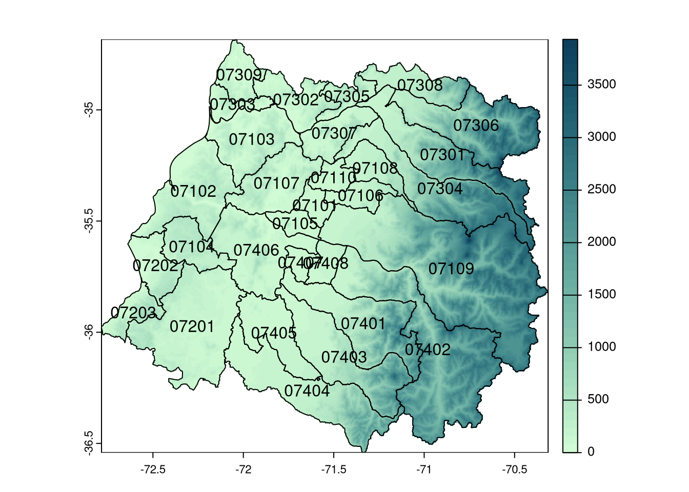
mapsf provides fairly flexible map creation functionality for overlaying layers of map information on a graphics output device, following the same order as above, but permitting the improvement of label positioning. Above, we set the palette to be used for elevation to "Dark Mint", which is the default for mapsf::mf_raster:
library(mapsf)
mf_raster(maule_elev, leg_pos="bottomleft",
leg_title="elevation (m)", leg_horiz=TRUE,
leg_size=0.8, leg_val_rnd=0)
mf_map(st_geometry(maule_sf), add=TRUE, lwd=2,
border="grey60", col="transparent")
mf_label(maule_sf, var="codigo_comuna", overlap=FALSE,
halo=2)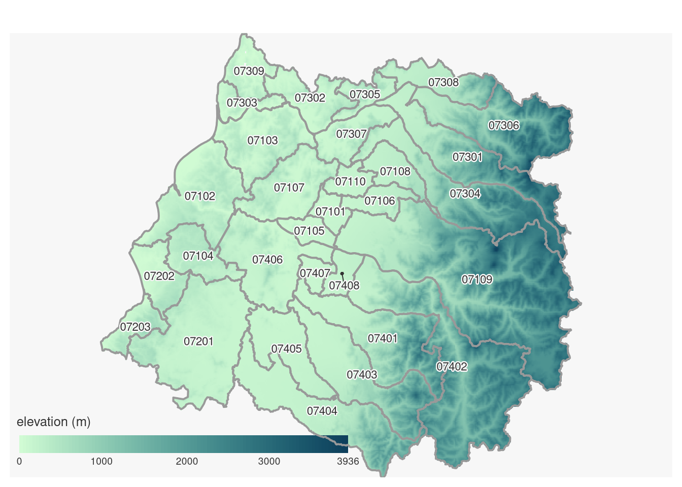
tmap is about to be upgraded, and is very concise in expressing map construction by adding successive layers to the output graphic with the + operator:
library(tmap)Breaking News: tmap 3.x is retiring. Please test v4, e.g. with
remotes::install_github('r-tmap/tmap')tm_shape(maule_elev) + tm_raster(n=15,
palette=rev(hcl.colors(7, "Dark Mint"))) +
tm_shape(maule_sf) + tm_borders() +
tm_text("codigo_comuna")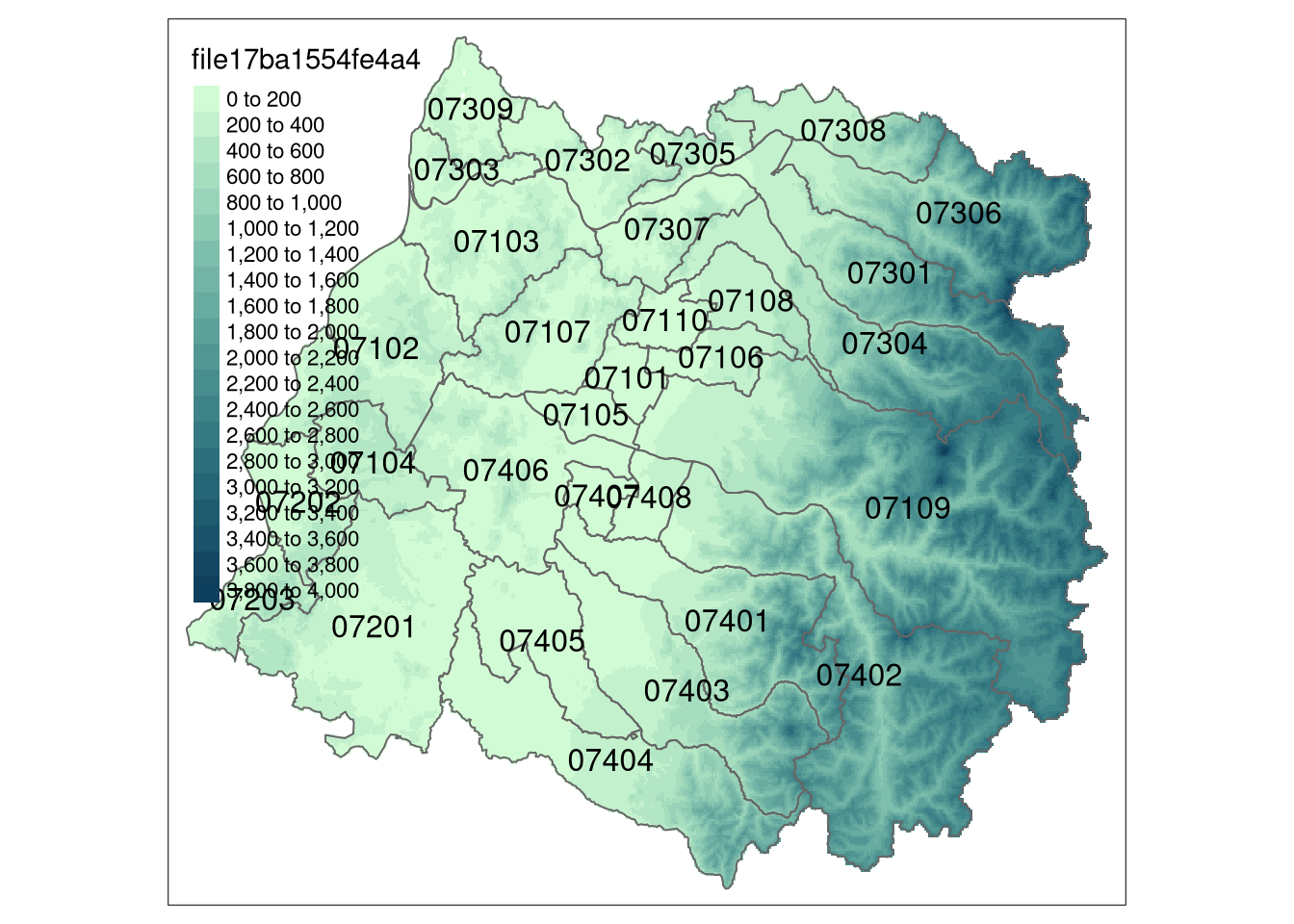
Using the simplest approach, we can plot the positions of the take-away outlets registered for Talca city in OpenStreetMap, and see that they are very clustered within the boundary of the municipality:
plot(st_geometry(talca_sf))
plot(st_geometry(talca_takeaways), pch=4, col=3,
cex=2, lwd=2, add=TRUE)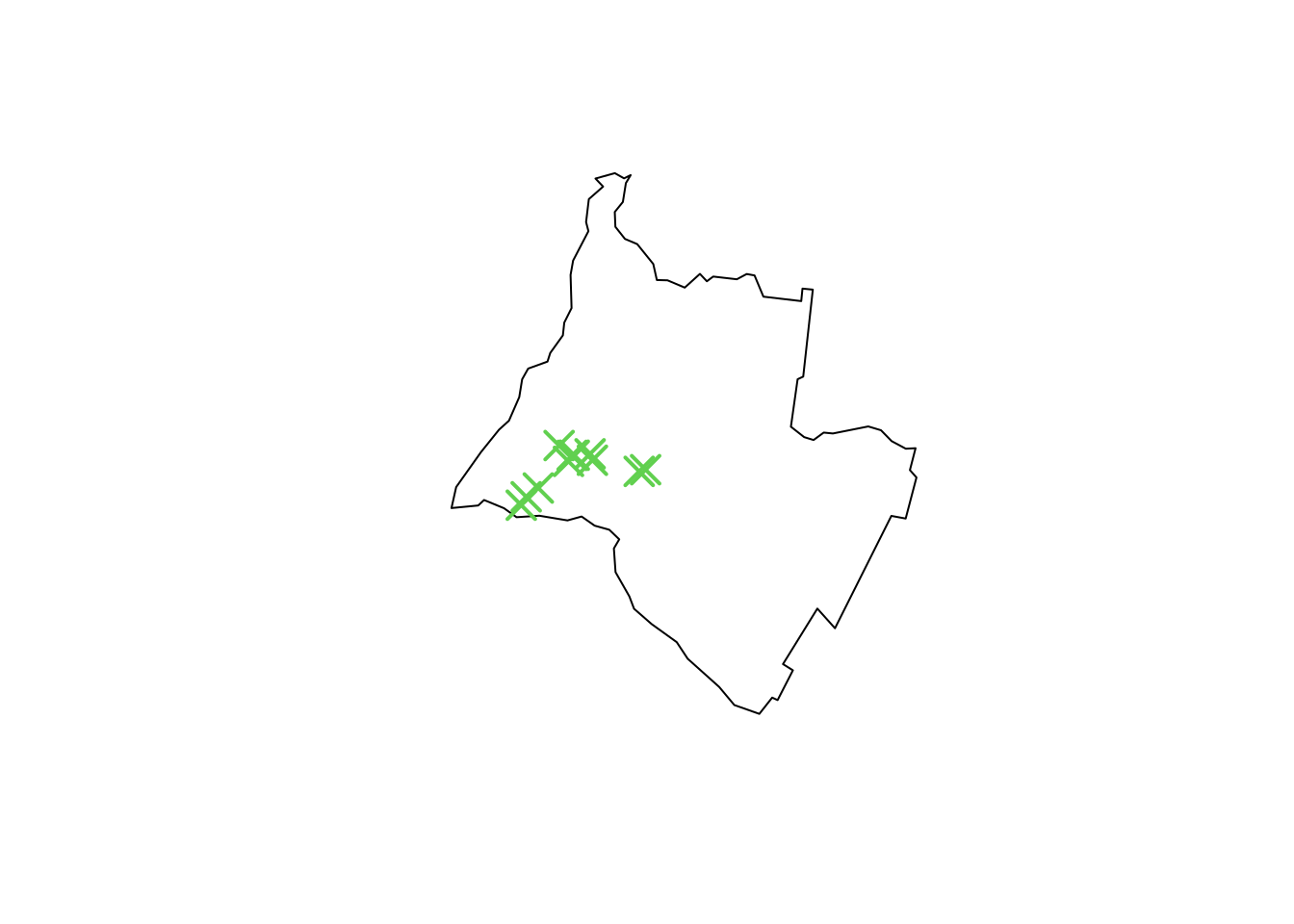
Since it would be very useful to obtain more locational context, we can use mapview to view the take-away outlets on a web map background, so that we can interact with the point locations. The mapview methods convert the object to be displayed to "OGC:WGS84" if necessary, then to Web Mercator for display:
library(mapview)
mapview(talca_takeaways)Interactive map of take-away outlets in Talca
Moving to the data set for municipalities in the Polish voivodeship of Pomerania, we can attempt to show the density variable on an interactive map:
library(mapview)
mapview(pom5, zcol="density")Interactive map of Pomeramia municipalities from rgugik, population density per square kilometre
As may be seen in the interactive map, the municipality boundaries do match the Baltic sea coastline quite well, but the jurisdiction of the municipalities extends to some coastal waters in the Gulf of Gdańsk and Zalew Wiślany; we did after all download administrative municipality boundaries using rgugik. We need to find another source of boundaries that agree with the coastline, and then need to take the intersection of the two sets od polygons, leaving only areas present in both. giscoR provides access to boundaries for European NUTS regions, in geographical coordinates by default. We then need to transform to the Transverse Mercator projection used for the download from rgugik before carrying out the intersection:
library(giscoR)
pom_gisco <- gisco_get_nuts(year="2021", resolution="01",
spatialtype="RG", nuts_id="PL63")
pom_gisco_tm <- st_transform(pom_gisco, "EPSG:2180")
pom6 <- st_intersection(pom5, pom_gisco_tm)Warning: attribute variables are assumed to be spatially constant throughout
all geometriesOn occasion, topological operations on two objects like st_intersection fail because the two geometries have different coordinate reference systems, in which case, st_transform should be used first to bring them into agreement. If in any topological operation or predicate (such as a query like st_intersects), it is found that a geometry is invalid, for example the self-intersection of a polygon boundary, use st_make_valid on the invalid object. It can be the case that the geometry cannot be repaired, as some data providers do not check the provided geometries for validity. Since an intersection operation can yield points and lines as well as polygons, we can check the input and output geometries and re-establish their original geometry types; in this case only polygons and multipolygons were output:
pom5 |> st_geometry_type() |> table() -> tab5; tab5[tab5>0]MULTIPOLYGON
123 pom6 |> st_geometry_type() |> table() -> tab6; tab6[tab6>0]
POLYGON MULTIPOLYGON
119 4 pom6 |> st_cast("MULTIPOLYGON") -> pom6Since the areas of some municipalities have now changed, we need to re-caluclate both areas and densities:
pom6 |> st_area() |>
units::set_units("km2") -> pom6$area_km2
pom6 |> st_drop_geometry() |>
subset(select = c(pop, area_km2)) |>
apply(1, function(x) x[1]/x[2]) -> pom6$densityAs can be seen from the figure below, the graphical representation is now more legible; coastlines and boundaries are typically read as contextual location information.
mapview(pom6, zcol="density")Interactive map of Pomeramia municipalities from rgugik, corrected population density per square kilometre
Two minor points before we move on, first that the distribution of the variable which we want to map does matter. The population density of Pomeranian municipalities is far from being symmetric, as this density plot shows:
plot(density(pom6$density))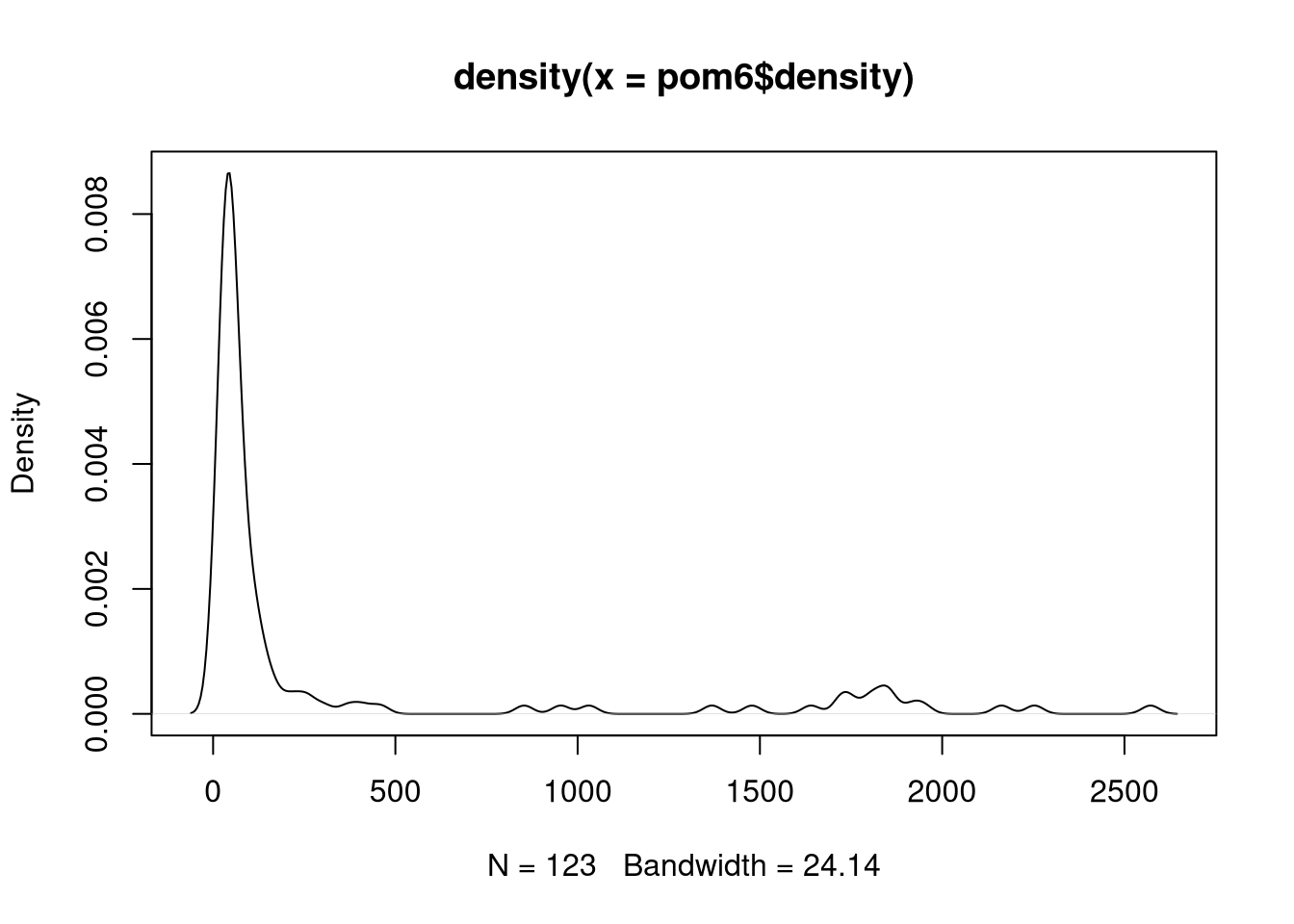
In this case, in thematic cartography we should create class intervals for display using quantiles or other suitable methods. mapsf provides a geometric progression "geom" method for creating class intervals for skewed variables:
mf_map(pom6, var="density", type="choro", breaks="geom",
nbreaks=7)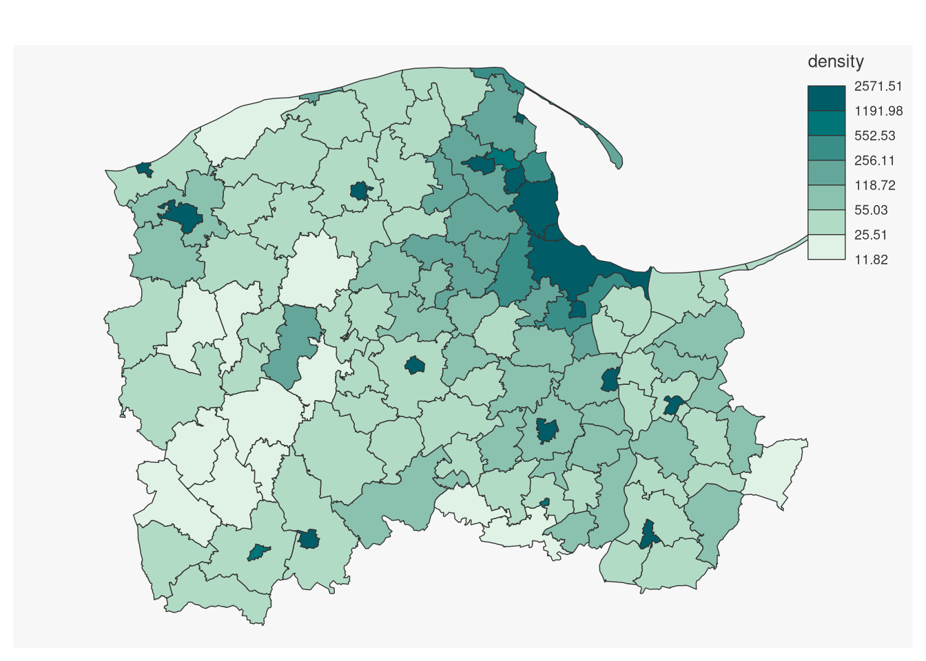
The choice of breaks style does matter for communicating the important traits of the variable in question in thematic cartography, here as a choropleth map.
The second display problem is associated with showing the kind of classes implied by the data. For a categorical variable and few classes, the classes are taken from the categories, and unlike the examples above using sequential palettes, this uses a qualitative palette:
mf_map(pom6, var="type", type="typo")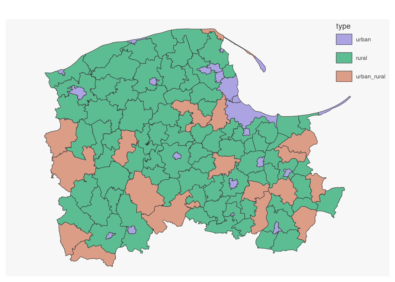
When the variable is crosses a specified mid-point, like regression residuals, a sequential palette is not appropriate, and a diverging palette should be chosen. tmap::tm_fill attempts to make reasonable choices in this situation; here the deviance of the proportion of the municipality population less than 16 years old from its mean:
pom6$young <- 100*(pom6$m_u15 + pom6$f_u15)/pom6$pop
pom6$young_res <- residuals(lm(young ~ 1, data=pom6))tm_shape(pom6) + tm_fill("young_res", style="quantile",
n=11, midpoint=0, palette="RdBu") + tm_borders()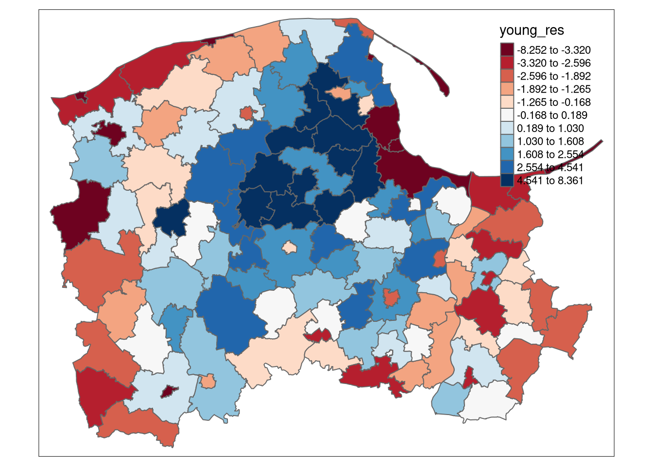
library(mapview)
mapview(gd_takeaways)Interactive map of take-away outlets in Gdańsk
For the present, we will only consider the reading and writing of spatial vector data using functions from sf: st_read and st_write. Further, while it is still regretably the case that many organisations still use the "ESRI Shapefile" (actually most often a bundle of at least four files) for sharing data, the GeoPackage format, "GPKG", should be preferred because it represents CRS properly, does not restrict field (variable) names to 10 characters, does use multibyte characters, and does store numerical fields in binary rather than text format. For commonly used formats, the format-specifiic driver is chosen from the file extension:
fn <- paste0(io_dir, "/pom6.gpkg")
if (file.exists(fn)) tull <- file.remove(fn)
try(st_write(pom6, fn))Writing layer `pom6' to data source `Input_output/pom6.gpkg' using driver `GPKG'
Creating field FID failed.
Error in eval(expr, envir, enclos) : Layer creation failed.Unfortunately, our intersection of the GISCO voivodeship outline added a number of variables to the data set, including one called "FID" , which is a reserved word for many spatial data formats, meaning “Feature IDentifier”, and must be an integer. Now it is a character vector, so we replace it by a compliant integer vector with unique values; we could also have dropped it:
str(pom6$FID) chr [1:123] "PL63" "PL63" "PL63" "PL63" "PL63" "PL63" "PL63" "PL63" "PL63" ...pom6$FID <- 1:nrow(pom6)
st_write(pom6, dsn=fn)Writing layer `pom6' to data source `Input_output/pom6.gpkg' using driver `GPKG'
Writing 123 features with 31 fields and geometry type Multi Polygon.To read, st_read will try to identify the format and use the appropriate driver automatically; if the data source containd multiple layers, the first will be read by default:
pom6a <- st_read(dsn=fn)Reading layer `pom6' from data source
`/home/rsb/und/PG_AGII_2sem/Input_output/pom6.gpkg' using driver `GPKG'
Simple feature collection with 123 features and 30 fields
Geometry type: MULTIPOLYGON
Dimension: XY
Bounding box: xmin: 350923.1 ymin: 626314.8 xmax: 542027.9 ymax: 774909.2
Projected CRS: ETRF2000-PL / CS92When we do a simple check to see if output and input are identical - and find that they are not:
isTRUE(all.equal(st_geometry(pom6), st_geometry(pom6a)))[1] FALSEWhen written to the external format, the order of the columns changes, as the geometry column is moved to the end on reading. This re-orders the columns, which contain the same information as before but the order differs:
names(pom6) [1] "TERYT" "NAME" "Nazwa"
[4] "m_u15" "f_u15" "m_15_64"
[7] "f_15_59" "m_o65" "k_o60"
[10] "type" "pop" "area_km2"
[13] "density" "farm" "non_farm_business"
[16] "non_farm_wages" "pension" "other_non_wage"
[19] "dwellings" "COAST_TYPE" "FID"
[22] "MOUNT_TYPE" "NAME_LATN" "CNTR_CODE"
[25] "NUTS_ID" "LEVL_CODE" "URBN_TYPE"
[28] "NUTS_NAME" "geo" "geometry"
[31] "young" "young_res" names(pom6a) [1] "TERYT" "NAME" "Nazwa"
[4] "m_u15" "f_u15" "m_15_64"
[7] "f_15_59" "m_o65" "k_o60"
[10] "type" "pop" "area_km2"
[13] "density" "farm" "non_farm_business"
[16] "non_farm_wages" "pension" "other_non_wage"
[19] "dwellings" "COAST_TYPE" "MOUNT_TYPE"
[22] "NAME_LATN" "CNTR_CODE" "NUTS_ID"
[25] "LEVL_CODE" "URBN_TYPE" "NUTS_NAME"
[28] "geo" "young" "young_res"
[31] "geom" In addition, the "area_km2" column loses its units definition, and the "type" column becomes a character vector, not a factor. Such differences are trivial and to be expected, but imply that if an object is to shared with collaborators, any shared script should use the object as read from file, especially if column order rather than column names are used in analysis. After reading, we can restore the representation of the columns before starting work:
pom6a$type <- factor(pom6a$type)
pom6a$area_km2 <- units::set_units(pom6a$area_km2, "km2")