4.1 Using spdep to create neighbour and weights objects
Chapter 14 of Pebesma and Bivand (2023) provides a fairly up-to-date account of how one may construct "nb" neighbour objects, and from these "listw" weights objects. In the following chapters, these objects will be used extensively in modelling, and will often be referred to as spatial weights matrices. While their description in terms of linear algebra as matrices is reasonable, their representation as dense n by n matrices is much less reasonable, as in most cases, only a very few elements of such a matrix are non-zero. This means that sparse representations are certainly preferable in terms of storage and efficiency, and repeated multiplication by zero is simply wasteful. "nb" neighbour objects, and "listw" weights objects are sparse representations, where the "nb" object records which objects j are neighbours of i for each i, and "listw" objects add in the weights assigned to each such i-j relationship.
We will use the spdep package to construct neighbour objects for the 123 Pomeranian municipalities. Since we have the boundaries of the municipalities, we can see which municipalities share boundary segments, known as rook contiguity; we add identifiers to the output object, now only to show it can be done, but later for use in out-of-sample prediction among other uses:
library(sf)
Linking to GEOS 3.12.1, GDAL 3.9.0, PROJ 9.4.0; sf_use_s2() is TRUE
Neighbour list object:
Number of regions: 123
Number of nonzero links: 504
Percentage nonzero weights: 3.33135
Average number of links: 4.097561
2 regions with no links:
2206011 2212053
7 disjoint connected subgraphs
If we slacken our definition of contiguity to simply sharing one boundary point, to queen contiguity, we see that the problems detected here of two no-neighbour municipalities and seven disjoint subgraphs remain:
Neighbour list object:
Number of regions: 123
Number of nonzero links: 504
Percentage nonzero weights: 3.33135
Average number of links: 4.097561
2 regions with no links:
2206011 2212053
7 disjoint connected subgraphs
One possible reason for such problems is that boundaries provided by public agencies are accurate enough for their purposes, but where shared boundary points are not exactly identical. If we pass a very small distance, here one-hundredth of a millimetre, as a snap distance, the problems are resolved:
Neighbour list object:
Number of regions: 123
Number of nonzero links: 614
Percentage nonzero weights: 4.058431
Average number of links: 4.99187
We can also see that in this case the rook and queen definitions lead to the same neighbour object; differences are more often seen in US tracts or counties with grid-like boundaries where four entities meet at a single point.
By definition, contiguity neighbours, like distance threshold neighbours are symmetric, that is if i is a neighbour of j, j must be a neighbour of i. This is only rarely the case when defining neighbours as the k-nearest points. Asymmetric neigbours lead to directed graphs, which can also be handled, but which need subsequent numerical special treatment. There may be substantive reasons for choosing asymmetric neighbours, but it is probably a good idea to spell out the reasons clearly.
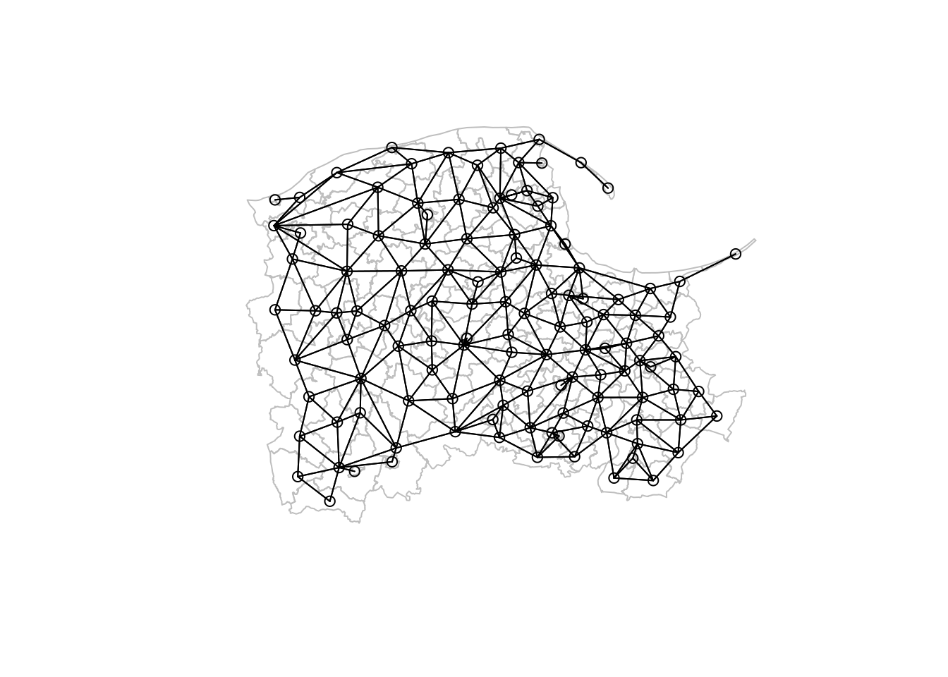
It is important to establish whether no-neighbour entities really have no neighbours because in matrix terms they lead to columns and rows with only zero values. Some methods become poorly defined if observations “drop out” of analysis in this way. For similar reasons, the detection of disjoint subgraphs, that is parts of the neighbour object that are unconnected from other parts of the object, jeopardises the outcome of modelling, as spatial processes cannot travel across the whole graph. The graph we have found now can be plotted, using st_point_on_surface internally to provide points to represent the polygons:
When choosing the five nearest neighbours as the neighbour criterion, with distance measured to suit the coordinate reference system of the point geometries, the outcome is most often asymmetric:
Neighbour list object:
Number of regions: 123
Number of nonzero links: 615
Percentage nonzero weights: 4.065041
Average number of links: 5
Non-symmetric neighbours list
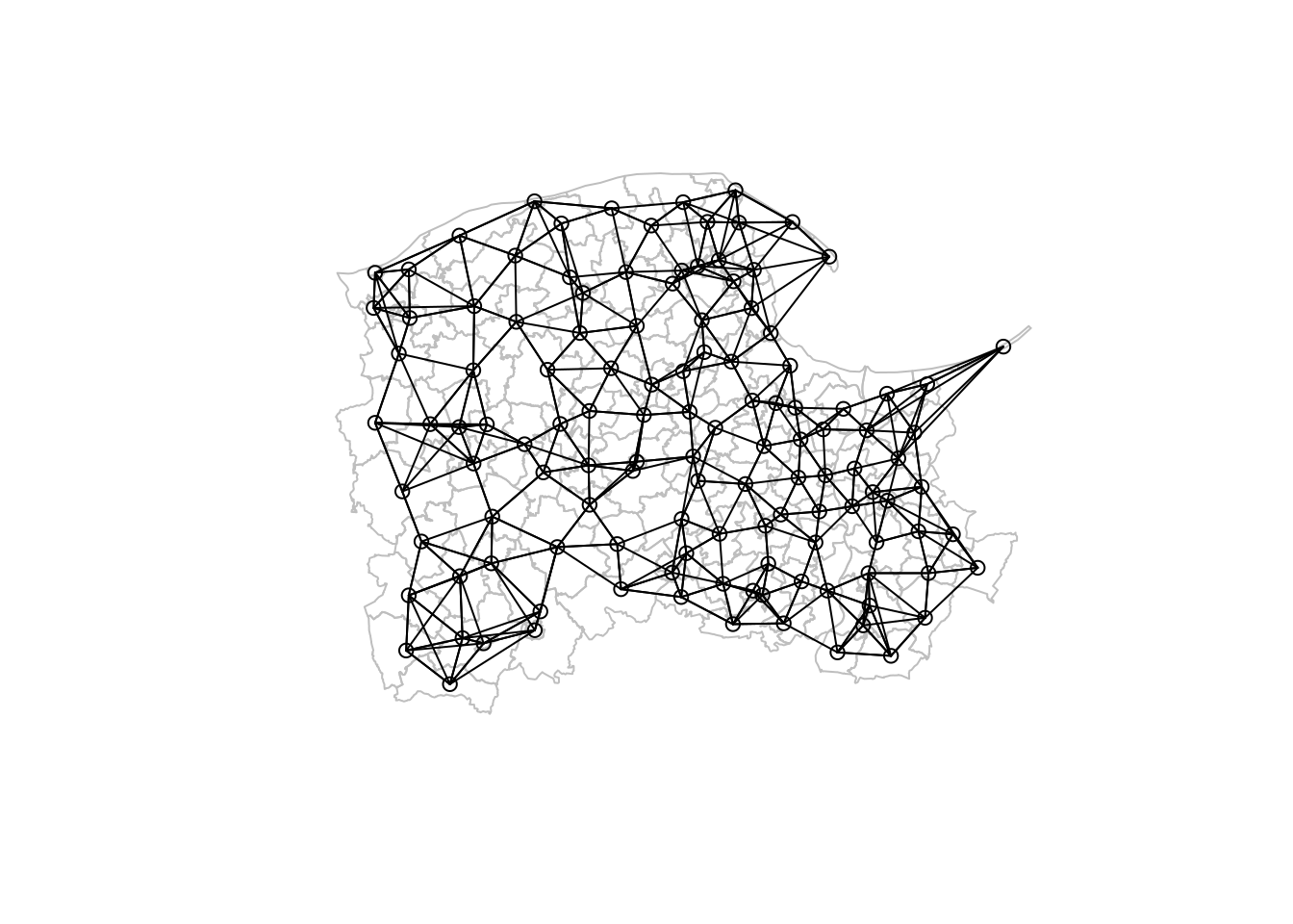
Five nearest neighbour object, Pomeranian municipalities, 2022
As the figure above shows, open coastal water is crossed by links between neighbours defined in this way. For the point support Gdańsk take-away outlets and five nearest neighbours, asymmetry is expected, but as with many distance measures, this case does raise the question of whether to measure distance in a distance metric or perhaps a time metric, because crossing a busy street takes more time than walking or cycling along a street:
Neighbour list object:
Number of regions: 160
Number of nonzero links: 800
Percentage nonzero weights: 3.125
Average number of links: 5
7 disjoint connected subgraphs
Non-symmetric neighbours list
As the figure below shows, the outlets are tightly clustered into disjoint subgraphs, but on more careful consideration, the outlets are multi-function, also serving drop-in customers. An outlet only offering take-away service might be located best near peak demand conditioned by the cost of property rental and transport accessibility, but most seem to sell to multiple markets: take-away, eat in restaurant, and delivery to customer. Maybe some compete on price, but cuisine may be a differentiator as well.
Characteristics of weights list object:
Neighbour list object:
Number of regions: 123
Number of nonzero links: 614
Percentage nonzero weights: 4.058431
Average number of links: 4.99187
Link number distribution:
1 2 3 4 5 6 7 8 9 10
7 10 12 14 30 22 16 8 3 1
7 least connected regions:
2203011 2206011 2210011 2211011 2211031 2212011 2213031 with 1 link
1 most connected region:
2206042 with 10 links
Weights style: W
Weights constants summary:
n nn S0 S1 S2
W 123 15129 123 57.8465 522.8508
The output of the summary method shows the same details as for the nb object, adding a tabulation by neighbour count, the weights style "W", meaning that the weights are standardised so that the sum of weights for each observation is unity:
pom_queen_lw$weights |>sapply(sum) |>unique()
[1] 1
In some modelling settings, the "B" binary zero-one style is preferred, and there are a number of alternative ways of specifying weights. Finally, if the neighbour object contains no-neighbour entities, the zero.policy argument to nb2listw may be used to indicate that zero weights are acceptable - the obvious alternatives are to exclude such entities, or to add neighbour links so that all entities have neigbours.
4.2 English garbage data set and weights construction
From the seventh lecture, we shall be using a data set from Bivand and Szymanski (1997) and Bivand and Szymanski (2000), extending results in SZYMANSKI and WILKINS (1993), SYMANSKI (1996) and Bello and Szymanski (1996). The question posed in the research reported in these articles is whether the costs of garbage collection in English local authority districts (which had a statutory obligation to collect garbage) were reduced when compulsory competitive tendering was introduced. Not all districts introduced compulsory competitive tendering at the same time, and some had not begun when data collection ceased. Of 366 districts, only 324 had completed at this point, and the data used relate to these districts. Since compulsory competitive tendering was implemented in different years, the data set reports real district net expenditure on garbage collection for the year before the implementation of compulsory competitive tendering (pre-CCT), and the year after (post-CCT).
As mentioned in Bivand and Szymanski (2000), the observations are agents, their boundaries do not change during the study period, and as entities they meet reasonable behavioural expectations. Revelli (2003), Brueckner (2003), Revelli (2006), Revelli and Tovmo (2007) and others engage with a literature including Case, Hines, and Rosen (1993) and Besley and Case (1995) concerning strategic interactions, of which yardstick competition may play a part. In Bivand and Szymanski (1997), the identification of residual spatial autocorrelation in the results given by Bello and Szymanski (1996) was used to develop a spatial yardstick competition framework, in which districts without compulsory competitive tendering were more likely to be influenced by the behaviour of their proximate neighbours than by general market conditions.
The data used in Bivand and Szymanski (2000) have been matched with simplified boundaries for English districts, and may be read in the usual way:
Reading layer `eng324s' from data source
`/home/rsb/und/PG_AGII_2sem/Datasets/cross section/garbage/eng324s.gpkg'
using driver `GPKG'
Simple feature collection with 324 features and 34 fields
Geometry type: MULTIPOLYGON
Dimension: XY
Bounding box: xmin: 134199 ymin: 11551 xmax: 655604 ymax: 657534
Projected CRS: OSGB36 / British National Grid
Showing which districts implemented compulsory competitive tendering and whether they awarded the contract to an outside bidder or to thir direct service organisation also shows the gaps, that is districts that had not implemented the policy by the end of data collection:
library(mapview)mapview(eng324, zcol="f_dso")
Direct service organisation chosen, compulsory competitive tendering, English districts
Naturally, the gaps lead to difficulties in creating a viable neighbour object:
Neighbour list object:
Number of regions: 324
Number of nonzero links: 1440
Percentage nonzero weights: 1.371742
Average number of links: 4.444444
3 regions with no links:
HEREFORD KENSINGTON & CHELSEA STEVENAGE
6 disjoint connected subgraphs
Three disticts have no neighbours, and there are 6 disjoint subgraphs. We can use k-nearest neighbours with small k to patch in the missing links, and make them symmetric:
Now we have a basis for work later on involving a data set used in published articles some time ago, but still relevant, as the entities are well-founded, and we have a micro-economic model for spillovers between entities.
Bello, Hakeem, and Stefan Szymanski. 1996. “COMPULSORY COMPETITIVE TENDERING FOR PUBLIC SERVICES IN THE UK: THE CASE OF REFUSE COLLECTION.”Journal of Business Finance & Accounting 23 (5-6): 881–903. https://doi.org/10.1111/j.1468-5957.1996.tb01157.x.
Besley, Timothy, and Anne Case. 1995. “Incumbent Behavior: Vote-Seeking, Tax-Setting, and Yardstick Competition.”American Economic Review 85 (1): 25.
Bivand, Roger, and Stefan Szymanski. 1997. “Spatial Dependence Through Local Yardstick Competition: Theory and Testing.”Economics Letters 55: 257–65.
———. 2000. “Modelling the Spatial Impact of the Introduction of Compulsory Competitive Tendering.”Regional Science and Urban Economics 30: 203–19.
Brueckner, Jan K. 2003. “Strategic Interaction Among Governments: An Overview of Empirical Studies.”International Regional Science Review 26: 175–88.
Case, Anne C., James R. Hines, and Harvey S. Rosen. 1993. “Budget Spillovers and Fiscal Policy Interdependence: Evidence from the States.”Journal of Public Economics 52 (3): 285–307. https://doi.org/10.1016/0047-2727(93)90036-S.
Pebesma, Edzer, and Roger Bivand. 2023. Spatial Data Science with Applications in R. Boca Raton, FL: CRC Press.
Revelli, Federico. 2003. “Reaction or Interaction? Spatial Process Identification in Multi-Tiered Government Structures.”Journal of Urban Economics 53: 29–53.
———. 2006. “Performance Rating and Yardstick Competition in Social Service Provision.”Journal of Public Economics 90: 459–75.
Revelli, Federico, and Per Tovmo. 2007. “Revealed Yardstick Competition: Local Government Efficiency Patterns in Norway.”Journal of Urban Economics 62: 121–34.
SZYMANSKI, STEFAN, and SEAN WILKINS. 1993. “Cheap Rubbish? Competitive Tendering and Contracting Out in Refuse Collection – 1981–88.”Fiscal Studies 14 (3): 109–30. https://doi.org/https://doi.org/10.1111/j.1475-5890.1993.tb00489.x.