There is a large literature in disease mapping using conditional autoregressive (CAR) and intrinsic CAR (ICAR) models in spatially structured random effects. These extend to multilevel models, in which the spatially structured random effects may apply at different levels of the model (Bivand et al. 2017). In order to try out some of the variants, we need to remove the no-neighbour observations from the tract level, and from the model output zone aggregated level, in two steps as reducing the tract level induces a no-neighbour outcome at the model output zone level. Many of the model estimating functions take family arguments, and fit generalised linear mixed effects models with per-observation spatial random effects structured using a Markov random field representation of relationships between neighbours. In the multilevel case, the random effects may be modelled at the group level, which is the case presented in the following examples.
We follow Gómez-Rubio (2019) in summarising Pinheiro and Bates (2000) and McCulloch and Searle (2001) to describe the mixed-effects model representation of spatial regression models. In a Gaussian linear mixed model setting, a random effect u is added to the model, with response Y, fixed covariates X, their coefficients \beta and error term \varepsilon_i \sim N(0, \sigma^2), i=1,\dots, n:
Y = X \beta + Z u + \varepsilon
Z is a fixed design matrix for the random effects. If there are n random effects, it will be an n \times n identity matrix if instead the observations are aggregated into m groups, so with m < n random effects, it will be an n \times m matrix showing which group each observation belongs to. The random effects are modelled as a multivariate Normal distribution u \sim N(0, \sigma^2_u \Sigma), and \sigma^2_u \Sigma is the square variance-covariance matrix of the random effects.
A division has grown up, possibly unhelpfully, between scientific fields using CAR models (Besag 1974), and simultaneous autoregressive models (SAR) (Ord 1975; Hepple 1976). Although CAR and SAR models are closely related, these fields have found it difficult to share experience of applying similar models, often despite referring to key work summarising the models (Ripley 1981, 1988; Cressie 1993). Ripley gives the SAR variance as (Ripley 1981, 89), here shown as the inverse \Sigma^{-1} (also known as the precision matrix):
\Sigma^{-1} = [(I - \rho W)^\top(I - \rho W)]
where \rho is a spatial autocorrelation parameter and W is a non-singular spatial weights matrix that represents spatial dependence. The CAR variance is:
\Sigma^{-1} = (I - \rho W)
where W is a symmetric and strictly positive definite spatial weights matrix. In the case of the intrinsic CAR model, avoiding the estimation of a spatial autocorrelation parameter, we have:
\Sigma^{-1} = M = \mathrm{diag}(n_i) - W
where W is a symmetric and strictly positive definite spatial weights matrix as before and n_i are the row sums of W. The Besag-York-Mollié model includes intrinsic CAR spatially structured random effects and unstructured random effects. The Leroux model combines matrix components for unstructured and spatially structured random effects, where the spatially structured random effects are taken as following an intrinsic CAR specification:
\Sigma^{-1} = [(1 - \rho) I_n + \rho M]
References to the definitions of these models may be found in Gómez-Rubio (2020), and estimation issues affecting the Besag-York-Mollié and Leroux models are reviewed by Gerber and Furrer (2015).
More recent books expounding the theoretical bases for modelling with areal data simply point out the similarities between SAR and CAR models in relevant chapters (Gaetan and Guyon 2010; Lieshout 2019); the interested reader is invited to consult these sources for background information.
8.2 Some CAR examples with English garbage data
In spatial econometrics, CAR is not used, nor are binary spatial weights; they both are, however, extensively used in spatial epidemiology (disease mapping). The CAR model accounts for spatial autocorrelation in the residuals of a linear model by modelling that residual dependency in various ways. spatialreg provides spautolm using Maximum Likelihood (ML) including a "CAR" family member, but does not have a direct method for extracting the spatially structured random effect (SSRE) from the fitted model:
Call: spautolm(formula = form_pre, data = eng324, listw = lwB, family = "CAR")

Residuals:
       Min         1Q     Median         3Q        Max
-1.2458705 -0.1271315 -0.0082244  0.1395717  0.9975448

Coefficients:
                 Estimate Std. Error z value  Pr(>|z|)
(Intercept)    -5.2940330  1.4601452 -3.6257 0.0002882
log(units)      0.9890709  0.0374943 26.3793 < 2.2e-16
house          -1.7376836  0.3188845 -5.4493 5.058e-08
log(dens)       0.0032286  0.0129677  0.2490 0.8033847
Metroplondon    0.1181653  0.0765654  1.5433 0.1227517
Metropmetrop    0.0032977  0.0648167  0.0509 0.9594235
log(realWgPre)  0.5710435  0.2692001  2.1213 0.0338999

Lambda: 0.12806 LR test value: 20.119 p-value: 7.2757e-06
Numerical Hessian standard error of lambda: 0.01965

Log likelihood: 10.54415
ML residual variance (sigma squared): 0.051948, (sigma: 0.22792)
Number of observations: 324
Number of parameters estimated: 9
AIC: -3.0883
Nagelkerke pseudo-R-squared: 0.84639
Cressie (1993) gives the spatial component of the fit as \rho_{\mathrm{Err}} {\mathbf W} ({\mathbf y} - {\mathbf X}{\mathbf \beta}) (p. 564, eq. 7.6.31):
eng324$ranef_ml <- car1$fit$signal_stochastic
Hierarchical GLM hglm(Alam, Rönnegård, and Shen 2015) can be used for fitting a proper CAR model as a rand.family argument passing in the binary spatial weights coerced into a symmetric sparse matrix:
library(hglm)W <-as(lwB, "CsparseMatrix")car2 <-hglm(fixed=form_pre, random=~1|ID, data=eng324, family =gaussian(), rand.family=CAR(D=W))car2
Call:
hglm.formula(family = gaussian(), rand.family = CAR(D = W), fixed = form_pre,
    random = ~1 | ID, data = eng324)

---------------------------
Estimates of the mean model
---------------------------

Fixed effects:
   (Intercept)     log(units)          house      log(dens)   Metroplondon
  -5.256205728    0.982604641   -1.740287615    0.006107953    0.109398222
  Metropmetrop log(realWgPre)
   0.015926892    0.572707449

Random effects:
[1]  0.07512008 -0.01960200  0.14569011
...
[1] 0.11309920 0.05048601
NOTE: to show all the random effects estimates, use print(hglm.object, print.ranef = TRUE).

Dispersion parameter for the mean model: 0.03210403

Dispersion parameter for the random effects: 3.83044e+21

Estimation did not converge in 3 iterations

!! Observation 65 is too influential! Estimates are likely unreliable !!
The fitting algorithm does not converge, so no estimate of the spatial autoregressive parameter is returned; a warning is given that one observation is highly unusual:
as.character(eng324$NAME[65])
[1] "CITY OF LONDON"
As almost nobody lives there, the proportion of houses in pick-up points is only 0.21, far below the median of 0.93; other variables are less extreme. No provision is made for dropping the outlier, so we will keep it; the SSRE is provided:
eng324$ranef_hglm <-c(unname(car2$ranef))
Finally, an intrinsic CAR (here termed Markov Random Field, MRF) can be fitted with mgcv using gam with an "mrf" smooth, and a spatial neighbour object with names set on the object components to match the variable defining the random effects:
library(mgcv)
Loading required package: nlme
This is mgcv 1.9-1. For overview type 'help("mgcv-package")'.
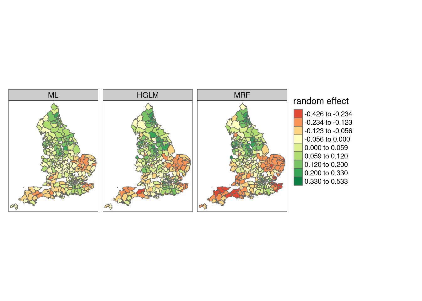
It is characteristic of work in disease mapping that the SSRE are mapped, and the maps are interpreted to learn whether the data collection could have been improved. It is not usual that work in spatial econometrics includes maps, and this difference has been noted critically by spatial statisticians. Here are comparative maps of the three output sets of SSRE:
library(tmap)
Breaking News: tmap 3.x is retiring. Please test v4, e.g. with
remotes::install_github('r-tmap/tmap')
Maps of spatially structured random effects, conditional autoregressive models
8.3 Simultaneous autoregressive models
There are many varieties of model fitting methods for CAR models, fewer for SAR. We can begin by using spautolm using Maximum Likelihood (ML) again, choosing SAR rather than CAR, but initially retaining the binary spatial weights:
Call: spautolm(formula = form_pre, data = eng324, listw = lwB, family = "SAR")

Residuals:
       Min         1Q     Median         3Q        Max
-1.1973371 -0.1330977  0.0042846  0.1472354  1.0226467

Coefficients:
                 Estimate Std. Error z value  Pr(>|z|)
(Intercept)    -5.2182355  1.4520462 -3.5937  0.000326
log(units)      0.9881039  0.0375060 26.3452 < 2.2e-16
house          -1.7196249  0.3196133 -5.3803 7.435e-08
log(dens)       0.0029204  0.0129370  0.2257  0.821401
Metroplondon    0.1254203  0.0767156  1.6349  0.102076
Metropmetrop    0.0093832  0.0648807  0.1446  0.885009
log(realWgPre)  0.5562152  0.2681111  2.0746  0.038026

Lambda: 0.073558 LR test value: 19.892 p-value: 8.1948e-06
Numerical Hessian standard error of lambda: 0.015158

Log likelihood: 10.4304
ML residual variance (sigma squared): 0.053275, (sigma: 0.23081)
Number of observations: 324
Number of parameters estimated: 9
AIC: -2.8608
Nagelkerke pseudo-R-squared: 0.84628
As row-standardised weights are much more common in spatial econometrics, let us switch (back) to them. First we see that the domain of the spatial coefficient depends on the spatial weights, and is the inverse of the range of the eigenvalues of the spatial weights matrix; this applies irrespective of the estimation method:
The value of the single spatial parameter is found by line search (univariate optimisation). In spautolm, the objective function includes the use of numerical inversion of the {\mathbf X}^\top{\mathbf A}{\mathbf X} matrix, where in the CAR case, {\mathbf A} = {\mathbf I} - \rho{\mathbf W}, but in the SAR case, it is {\mathbf A} = ({\mathbf I} - \rho{\mathbf W})^\top({\mathbf I} - \rho{\mathbf W}), using plug-in functions. Using spautolm, we get:
Call: spautolm(formula = form_pre, data = eng324, listw = lw, family = "SAR",
    control = list(pre_eig = e))

Residuals:
       Min         1Q     Median         3Q        Max
-1.2099474 -0.1382060 -0.0061752  0.1467393  1.0037329

Coefficients:
                  Estimate  Std. Error z value  Pr(>|z|)
(Intercept)    -4.99283719  1.49150170 -3.3475 0.0008154
log(units)      0.99637181  0.03760832 26.4934 < 2.2e-16
house          -1.73716260  0.31817206 -5.4598 4.766e-08
log(dens)       0.00052967  0.01256022  0.0422 0.9663626
Metroplondon    0.10864174  0.07912775  1.3730 0.1697549
Metropmetrop   -0.00633204  0.06608941 -0.0958 0.9236713
log(realWgPre)  0.50480257  0.27573061  1.8308 0.0671331

Lambda: 0.35401 LR test value: 19.988 p-value: 7.7912e-06
Numerical Hessian standard error of lambda: 0.072223

Log likelihood: 10.47868
ML residual variance (sigma squared): 0.05332, (sigma: 0.23091)
Number of observations: 324
Number of parameters estimated: 9
AIC: -2.9574
Nagelkerke pseudo-R-squared: 0.84632
spautolm outputs the standard error of the spatial coefficient based on the numerical Hessian to estimate the information matrix of the model. errorsarlm was written before spautolm, and yields very similar values, using for moderate n as in this case asymptotic standard errors:
In addition, output from errorsarlm offers the Hausman test (Pace and LeSage 2008); the SEM and OLS regression coefficients should be close to each other and significant divergence indicates model mis-specification; it seems difficult here to accept the null hypothesis of no difference:
Hausman.test(SEM_pre)
    Spatial Hausman test (asymptotic)

data:  NULL
Hausman test = 21.049, df = 7, p-value = 0.003699
8.4 Spatial econometrics models: pre-CCT examples
We have already fitted the SEM model using ML to the basic pre-CCT formula, partly based on our initial results, indicating that SEM was to be preferred to SLM, but without considering the inclusion of {\mathbf W}{\mathbf X}.
Use of Rao’s score tests only involve the fitting of least squares models, both OLS and SLX, but it is also possible to work back from the most complex model GNM, recalling its identification issues (using ML):
However, since GNM includes \rho_{\mathrm{Lag}} {\mathbf W}{\mathbf y}, presenting the conventional table of coefficient estimates is not appropriate, so we’ll stay with likelihood ratio tests, which depend on the models being compared being nested, and returning log-likelihood values:
where \ell(\theta_0) is the log-likelihood of the nested model, and \ell(\theta_1) of the encompassing model, and where the number of degrees of freedom for \chi^2 is the difference in the estimated parameter counts.
library(lmtest)
Loading required package: zoo
Attaching package: 'zoo'
The following objects are masked from 'package:base':

    as.Date, as.Date.numeric
lrtest(GNM_pre, SAC_pre)
Likelihood ratio test

Model 1: log(realNetPre) ~ log(units) + house + log(dens) + Metrop + log(realWgPre)
Model 2: log(realNetPre) ~ log(units) + house + log(dens) + Metrop + log(realWgPre)
  #Df LogLik Df  Chisq Pr(>Chisq)
1  14 17.361
2  10 10.887 -4 12.947    0.01154 *
---
Signif. codes:  0 '***' 0.001 '**' 0.01 '*' 0.05 '.' 0.1 ' ' 1
This test indicates that including {\mathbf W}{\mathbf X} to the SAC model to give an GNM model only yields a minor improvement in fit. Moving on, we fit the remaining models:
The LM test for residual spatial autocorrelation in the SLM model indicates that something in the {\mathbf W}{\mathbf X} is adding spatial autocorrelation to the residuals.
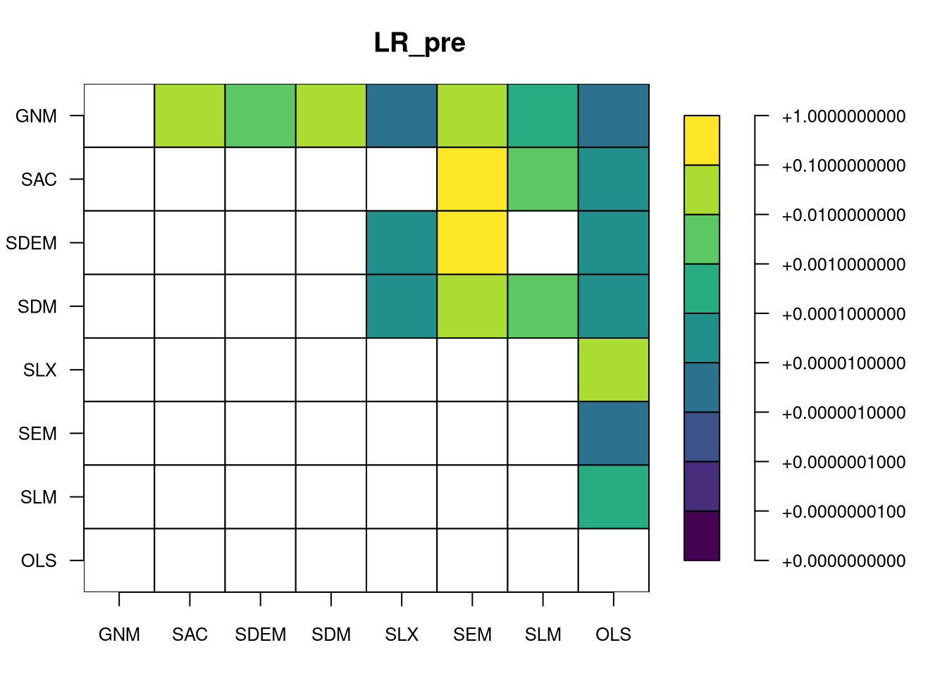
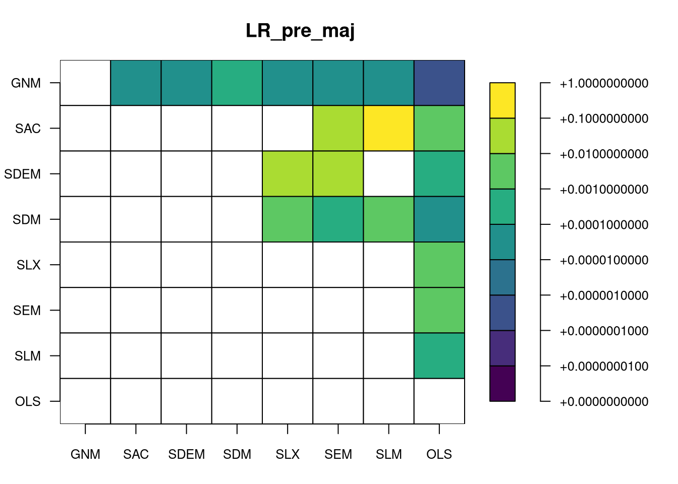
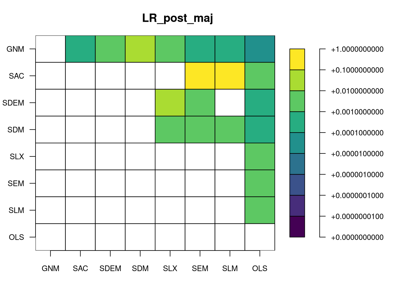
we now have eight fitted pre-CCT models, and can calculate the likelihood ratio tests between nested models. GNM nests all models, SAC nests SEM, SLM and OLS, SDEM nests SEM, SLX and OLS, SDM nests SLM, SLX and OLS (and SEM through the Common Factor \rho_{\mathrm{Err}} = - \rho_{\mathrm{Lag}}{\mathbf \beta}), and SEM, SLX and SLM nest OLS:
Heat map of likelihood ratio p-values, pre_CCT models
par(opar)
The figure shows that the only comparisons indicating minor improvement in fit by making the model more complex are from SEM to SDEM or SAC; it is not clear that adding the {\mathbf W}{\mathbf X} helps. In addition, the likelihood ratio does not penalise for the increased number of fitted paramters, unlike AIC and BIC, which penalise in increasing degree. The Akaike information criterion (AIC) is, where k is the parameter count:
The BIC scores put all of the models including {\mathbf W}{\mathbf X} behind those without, pointing to SEM, followed by SAC and SLM. The Bayesian information criterion (BIC) is, for n, the observation count:
So we might reasonably choose to proceed with SLM including political control, but will have to wait to present coefficient estimates, or rather the marginal effects, because SLM includes \rho_{\mathrm{Lag}} {\mathbf W}{\mathbf y}.
Alam, Moudud, Lars Rönnegård, and Xia Shen. 2015. “Fitting Conditional and Simultaneous Autoregressive Spatial Models in Hglm.”The R Journal 7 (2): 5–18. https://doi.org/10.32614/RJ-2015-017.
Besag, Julian. 1974. “Spatial Interaction and the Statistical Analysis of Lattice Systems.”Journal of the Royal Statistical Society. Series B (Methodological) 36: pp. 192–236.
Bivand, Roger, Zhe Sha, Liv Osland, and Ingrid Sandvig Thorsen. 2017. “A Comparison of Estimation Methods for Multilevel Models of Spatially Structured Data.”Spatial Statistics. https://doi.org/10.1016/j.spasta.2017.01.002.
Cressie, Noel A. C. 1993. Statistics for Spatial Data. New York: John Wiley & Sons.
Gaetan, Carlo, and Xavier Guyon. 2010. Spatial Statistics and Modeling. New York: Springer.
Gerber, Florian, and Reinhard Furrer. 2015. “Pitfalls in the Implementation of Bayesian Hierarchical Modeling of Areal Count Data: An Illustration Using BYM and Leroux Models.”Journal of Statistical Software, Code Snippets 63 (1): 1–32. https://doi.org/10.18637/jss.v063.c01.
Hepple, Leslie W. 1976. “A Maximum Likelihood Model for Econometric Estimation with Spatial Series.” In Theory and Practice in Regional Science, edited by I. Masser, 90–104. London Papers in Regional Science. London: Pion.
Lieshout, M. N. M. van. 2019. Theory of Spatial Statistics. Boca Raton, FL: Chapman & Hall/CRC.
McCulloch, Charles E., and Shayle R. Searle. 2001. Generalized, Linear, and Mixed Models. New York: Wiley.
Ord, J. Keith. 1975. “Estimation Methods for Models of Spatial Interaction.”Journal of the American Statistical Association 70: 120–26.